Our previous series, “Inside LLM serving: The journey of a token,” walked through how LLMs run quickly and reliably in production and traced the full path a user’s request takes from server to generated response. This post picks up where that series left off and turns to HyperCLOVA X SEED 8B Omni, Korea’s first omni-model—one that handles images and audio alongside text. We’ll share how we designed the serving architecture and tuned its performance to deliver it reliably in production.
Why omnimodal?
Our daily lives aren’t made up of text alone. When we have a conversation, we take in not just the words but also tone of voice, facial expressions, the context of the exchange, and visual cues from our surroundings—and when we respond, we naturally weave voice, expression, and situational language into what we say. Real-world communication is closer to exchanging multiple kinds of information at once. For AI to do meaningful work in real environments, then, it has to understand and generate not just text but visual and audio information—multiple modalities together.
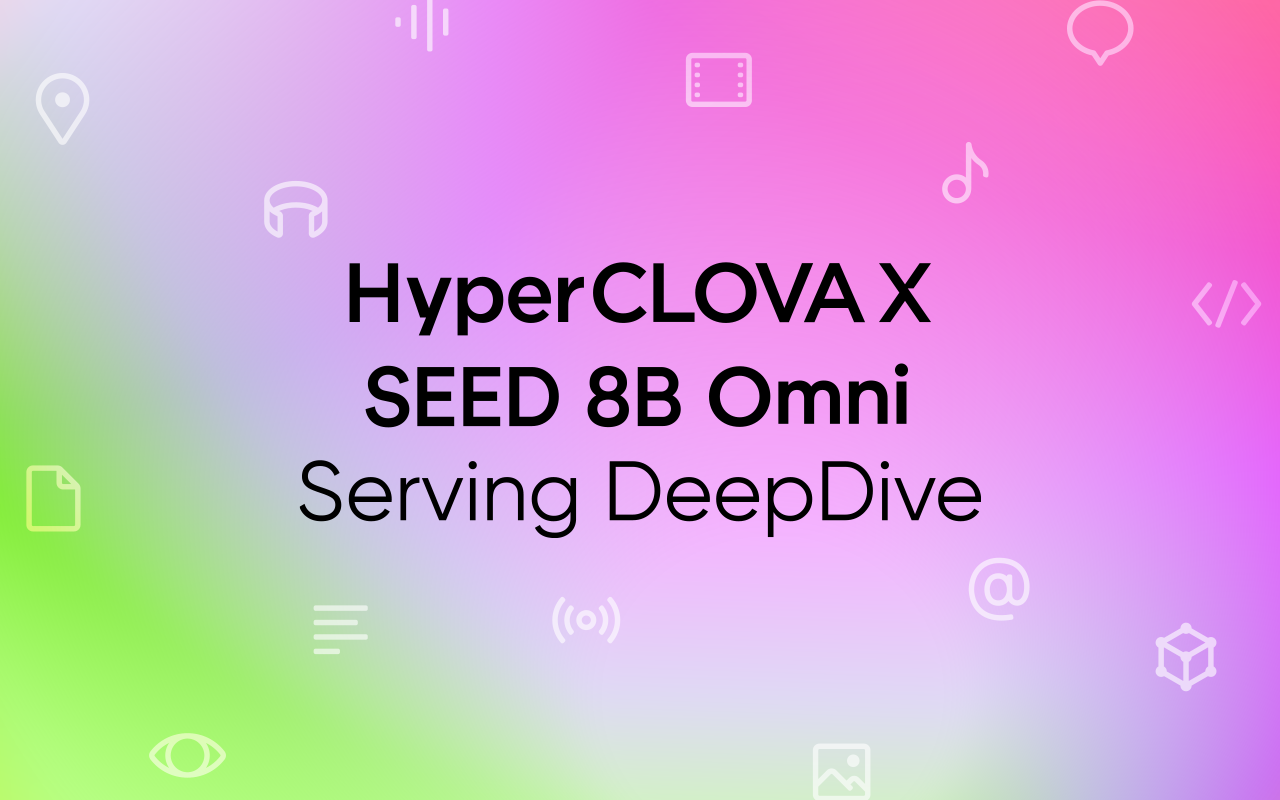
That’s where the idea of omnimodal comes in. An omnimodal model learns different kinds of data—images, audio, text—in a single semantic space, so it can understand and generate them in an integrated way rather than handling each in isolation. Concretely, the images and audio a user provides are converted by an encoder into representations the model can understand, and a decoder produces a response in whatever form fits the situation. The result is richer interaction that goes beyond text-centric responses to include images and audio.
▲ Source: NAVER Cloud HyperCLOVA X Team, “HyperCLOVA X 8B Omni,” arXiv:2601.01792, Jan. 2026.
In line with this, we developed HyperCLOVA X SEED 8B Omni. (For more, see HyperCLOVA X OMNI: Korea’s flagship AI on the road to omnimodality.) This post walks through how we designed the serving architecture and optimized performance to deliver this omnimodal model in production—fast and reliably?
System design: Splitting Encoder, Decoder, and LLM
Why a split architecture
HyperCLOVA X SEED 8B Omni is a single model with the Encoder and Decoder integrated into one structure. But in production, that structure hit a wall on resource efficiency. When only video-related requests were coming in, for example, the audio-processing parts sat idle inside the GPU, holding memory without doing anything. When video traffic grew and we had to scale out, only the video-processing parts actually needed more capacity—but the audio parts scaled along with them, multiplying the unused resources.
Wasted resources and cost weren’t the only issue. With Encoder, Decoder, and LLM all running inside one server, they competed for GPU resources, dragging overall performance down. To fix this, instead of bundling every function into one structure, we split the Encoder, Decoder, and LLM into independent servers.
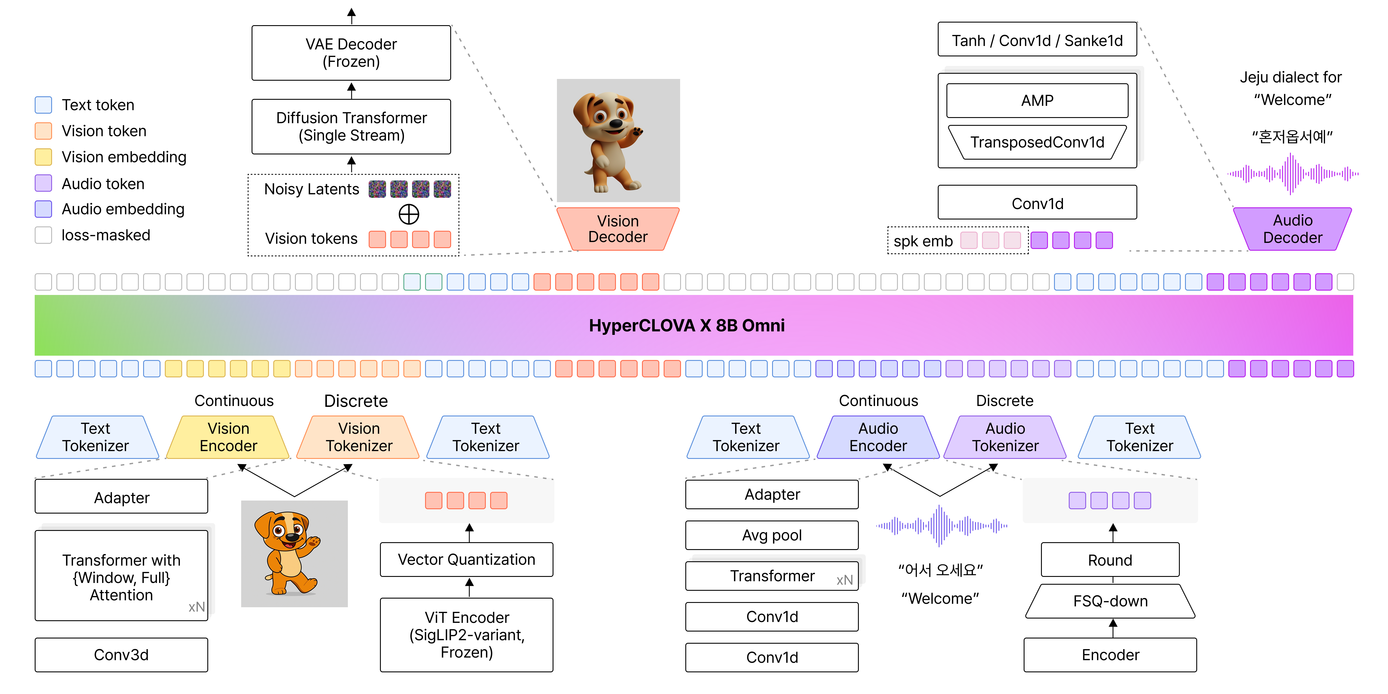
 ▲ Before (left) and after (right): splitting Encoder, Decoder, and LLM into separate servers.
The diagram makes the difference clearer. In the original architecture on the left, unused functions take up GPU space, so resources are used inefficiently—and the Vision Encoder and LLM compete for resources on the same GPU. With the separated architecture on the right, each component can use its GPU resources fully, and we can scale only the functions that actually need more capacity, sharply reducing waste.
Choosing an orchestration approach
Once the components were split, the next question was how to connect them. Wrapping each function in its own container and managing the lot with Kubernetes was an easy call—it’s close to an industry standard. From a system architecture perspective, though, we had to decide between an API Gateway-based service chaining approach and a central orchestrator approach.
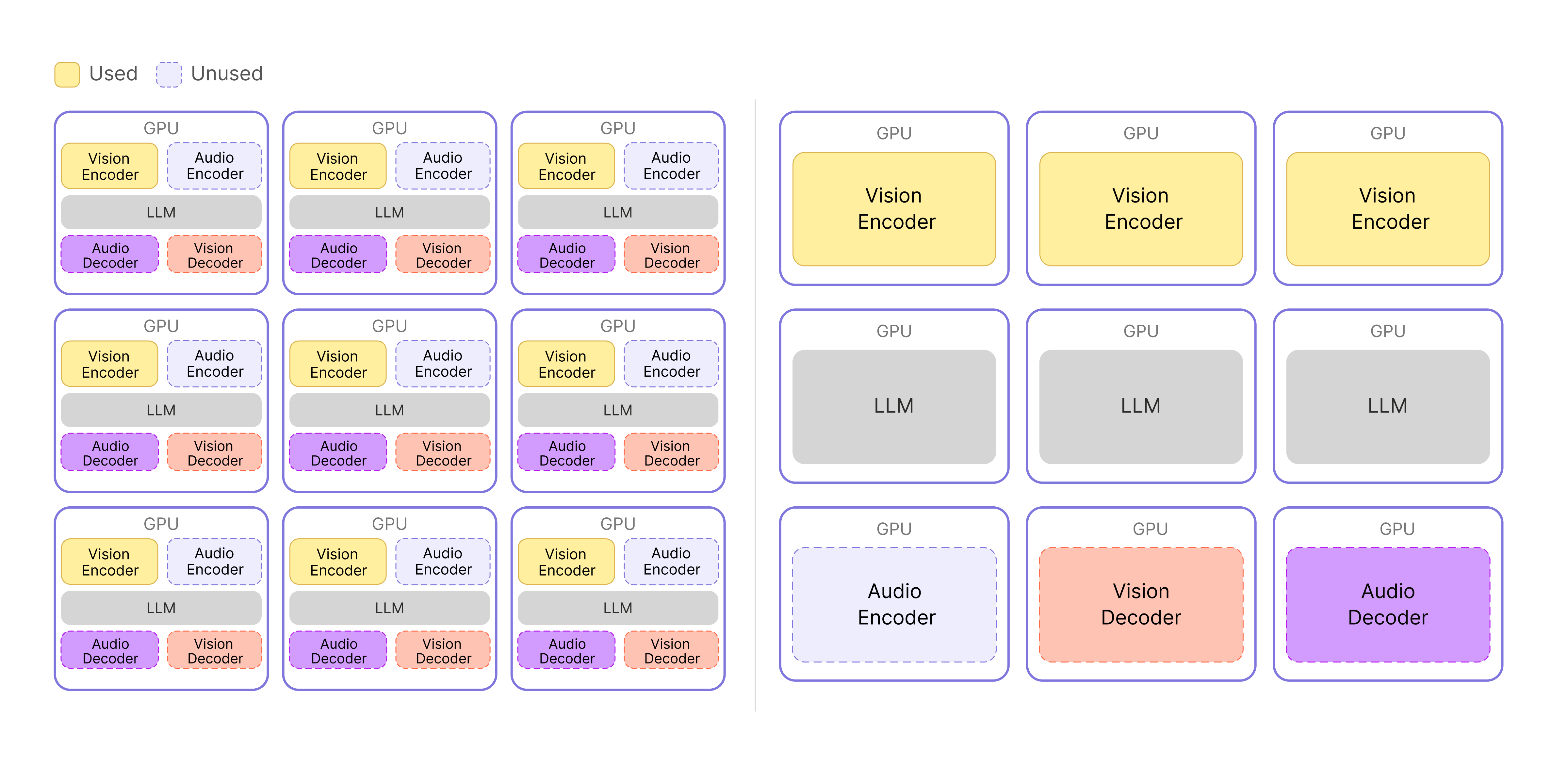
▲ Left: API Gateway with service chaining. Right: central orchestrator.
- API Gateway-based service chaining
Service chaining is flexible: when you need a new feature, you can extend the system by composing existing functions. But in our case, the omni-model was originally built as a single integrated structure, with the Encoder and Decoder tightly coupled to the LLM, so there wasn’t much need to extend by adding new connections. And on a tight schedule, choosing a structure with calls scattered across components carried a real risk: when something went wrong, tracing the call flow to debug it would get complicated, slowing down development overall.
- Central orchestrator
The central orchestrator approach concentrates all flow at a single point, which creates a single point of failure (SPOF) risk—if that point breaks, the whole system can be affected. Even so, it has a clear advantage: with the logic gathered in one place, you can see the flow at a glance, pinpoint problems quickly when they happen, and move fast.
We ultimately went with a central orchestrator, but kept its responsibilities as small as possible to minimize failure modes.
Designing the interfaces between components
With the LLM, Encoder, and Decoder split apart this way, how data moves between components becomes a key design question. We focused on clearly defining the inter-server communication and data formats as we worked out the API spec for each component.
For the LLM server, we prioritized compatibility and adopted the OpenAI Chat Completion API as-is—the de facto standard across the industry. We also made the Orchestrator follow the same spec so that requests could pass between client and LLM with no extra translation. The Orchestrator’s job, then, is to call the Encoder and Decoder based on the input data format and assemble each stage’s results back into the OpenAI Chat Completion API format.
The Encoder and Decoder, on the other hand, handle different kinds of data, so we designed separate APIs tailored to each role. The Encoder turns raw inputs like images or audio into token IDs or embedding vectors—the form the LLM can understand. The Decoder does the reverse: it takes token IDs generated by the LLM and uses them to produce the final image or audio.
One more piece needed extra design work: passing the embeddings generated by the Encoder to the LLM. We initially tried to handle this inside the model with a plugin, but the embedding-passing path got complicated and code maintenance and debugging suffered. So we opted to keep the structure simpler: send the embeddings from the Encoder to the LLM server through the Data Plane, then combine them with the input vectors the LLM is processing (the embeddings derived from tokens) and inject them directly as model input. This kept the data flow clearer while reducing complexity.
We’ll look at how data actually moves through the Data Plane in the next section.
Why we chose Object Storage as the Data Plane
Beyond the interfaces themselves, we needed to design how the intermediate artifacts would actually move around. In omnimodal serving, performance is directly tied to how those artifacts—embedding vectors, token IDs, and the like—get passed between Encoder, LLM, and Decoder. As described earlier, video and audio data is converted into these forms as it passes through the Encoder. We treated those artifacts as assets—things that could be pulled out and reused across servers and stages—rather than as throwaway temporary data.
That led us to choose a shared pathway for moving and storing data across the system: Object Storage (OBS), serving as the Data Plane. This gave us one path for both transfer and caching, instead of separate mechanisms for each.
The implementation is simple. We serialize the Encoder’s output into a file and upload it to OBS. After that, instead of passing the data itself around, we pass only a pointer that says where the data lives—the actual data is fetched on demand. The object key is like a label on the stored file, and a presigned URL is a temporary link that grants access for a limited window. The LLM or Decoder reads this address and fetches the data straight from storage when it needs it.
This gave us several benefits:
- We can handle any artifact through the same interface, regardless of its size or format.
- Because the data isn’t tied to a specific server, the system stays flexible when work is distributed across servers.
- In multi-turn conversations, intermediate results that have already been generated can be reused, saving repeat computation along with time and compute.
- Since every component shares the same Object Storage, even when a follow-up request lands on a different server, the same data can be reliably retrieved.
Object Storage ended up being more than just storage—it became the core Data Plane that lets us reliably manage intermediate artifacts in omnimodal serving and reuse them whenever they’re needed.
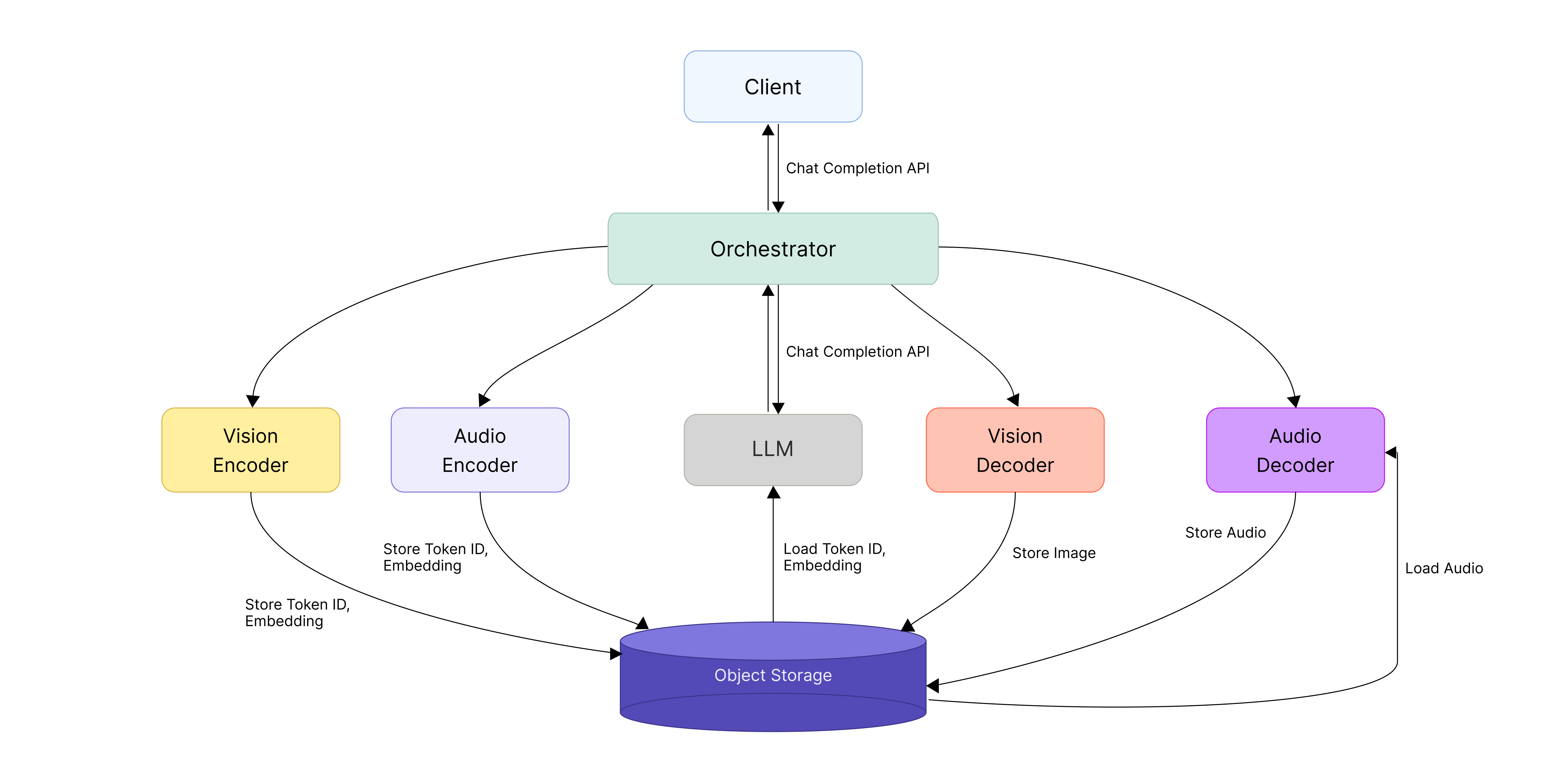
▲ System architecture for omni-model serving
Maximizing KV cache reuse with llm-d
Why we adopted llm-d
vLLM performs well on a single server, but in a distributed setup with multiple servers it was hard to fully tap into the speedup that comes from KV cache reuse—the technique that accelerates an LLM by storing earlier computation results and reusing them.
When an LLM processes a prompt, it stores the computation results from earlier tokens as a KV cache, and if the same prefix shows up again, it reuses them to skip redundant work. The catch is that the KV cache lives only in each server’s local memory. So if requests sharing the same prefix get spread across different servers, they can’t reuse the cache and have to recompute. The upshot was that adding more servers didn’t deliver the performance gains we expected. What mattered wasn’t splitting requests evenly—it was routing each request to the server that already held the relevant context (prefix).
- Prefix: the front portion of an input prompt that several requests share in common
e.g., a system prompt or prior conversation history that gets included repeatedly
Our solution was llm-d. llm-d is a scheduler that routes requests by considering both each server’s KV cache state and its current load, sending requests with the same prefix to the same server whenever possible to maximize cache reuse.
Challenges in adopting llm-d
This came with a few challenges, though. Before we could roll llm-d into production, we had to work through a handful of structural issues across both the routing layer and how requests were processed.
We faced three main challenges:
- Each model server used a different entry point, making it hard to apply a unified routing policy.
- We needed to route based on the model information in the request body, but llm-d didn’t offer that capability out of the box.
- We had to factor in not just cache utilization but also server load.
On top of that, the early llm-d was designed around Hugging Face, so we had to modify the relevant code ourselves to make it work with our in-house Omni model. Adopting llm-d ended up being less about plugging in a feature and more about working through the constraints of our serving environment one by one and reshaping the structure to fit.
1) Moving to a unified gateway with shared routing
The first thing we had to fix was the entry point (ingress) structure, which was split across model servers.
With entry points scattered across servers, it was hard to apply a routing policy that took KV cache state into account in any consistent way, and operational complexity kept climbing. To fix this, we consolidated the model servers behind a single shared gateway. That let us manage routing policy centrally and laid the groundwork for stably applying llm-d-based routing on top.
2) Body-based model routing
The next challenge was deciding which model a request should go to.
In our environment we needed to pick the model server group (InferencePool) based on the model name in the request body, but llm-d didn’t support body-based routing out of the box.
To work around this, we used EnvoyFilter and HttpRoute—components for transforming requests and controlling routing.
Here’s how it works:
- Step 1: EnvoyFilter pulls the model information out of the request body and passes it to a custom ModelResolver we built.
- Step 2: ModelResolver adds that information to a header.
- Step 3: HttpRoute then routes to the appropriate model server group based on that header value.
3) Picking a model server in a distributed environment
Even after the model was chosen, it still mattered which specific server within that model’s group (InferencePool) the request landed on. We needed to factor in each server’s load, so simply picking the server with the highest cache utilization wasn’t enough. To balance the two, we tuned the scoring items and weights to reflect both KV cache utilization and server load (queue):
- weight: 3.0 – pluginRef: kv-cache-utilization-scorer
- weight: 2.0 – pluginRef: queue-scorer
- weight: 2.0 – pluginRef: max-score-picker
Here’s what each weighted item does:
- kv-cache-utilization-scorer: evaluates how likely a server is to reuse the KV cache because it has handled similar requests before. We set this weight highest (3.0) because it has the biggest impact on performance.
- queue-scorer: reflects each server’s load based on the length of its current request queue
- max-score-picker: selects the server with the highest final score
llm-d evaluates each server (replica) against multiple criteria, computes a weighted score, and picks the server with the highest score. With the criteria above, we put together a balanced routing strategy that prefers servers where the cache can be reused while also taking server load into account, so requests don’t pile up on any one server.
Here’s the full flow of the improvements we’ve described so far:
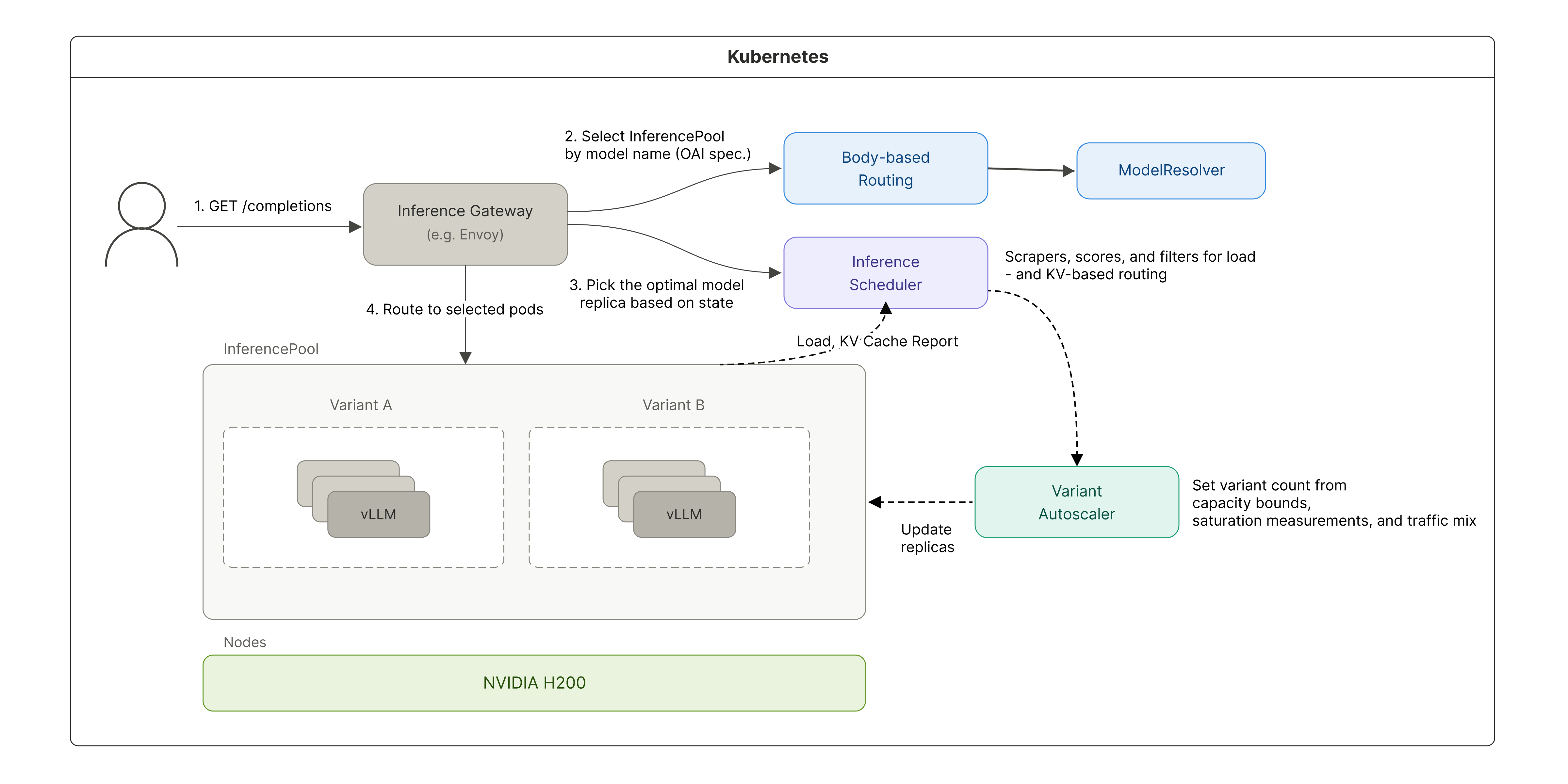
▲ Distributed inference architecture with llm-d applied
Results
These changes let us roll out llm-d into our production serving environment reliably. Throughput improved by 2.1x, and KV cache utilization climbed from a previous range of 25–45% to over 90%. We also contributed the improvements we made along the way back to the open-source project.
Encoder/Decoder compute optimization
Beyond the system architecture and distributed-side optimizations, we also went after the compute time of the Encoder and Decoder components themselves. The compute characteristics of each component look like this:
- Vision/audio Encoder, LLM prefill: compute-bound operations that batch the input together
- LLM decode: a memory-bound operation that has to load the full weights for every token
- Vision Decoder: a compute-bound operation that prefills an 8K sequence N times without a KV cache
- Audio Decoder: a compute-bound operation handled in a single prefill
Vision Encoder: From 784 Conv3D calls down to one
OmniServe is the multimodal inference system for HyperCLOVA X SEED 8B Omni.
Early on, FlashAttention2—the feature that speeds up attention computation—was disabled because the numeric format (dtype) didn’t match. The highway was open, but the on-ramp was blocked, so traffic was stuck on side roads. Once we fixed the dtype, FlashAttention2 started working properly, and at that point a single image’s Vision Encoder forward pass took 43 ms. Here’s how we cut it further from there.
PatchEmbed was the bottleneck
Profiling showed that 68% of total compute was being spent in PatchEmbed—the first stage, which splits an image into small patches the AI can understand and turns each patch into a vector.
The problem was how it was processing them. The image was being split into 14×14 patches, and Conv3D was being called separately on each patch. Conv3D is an operation that extracts features from an image—and we were applying a filter that could have run once over the whole picture to hundreds of fragments individually.
For high-resolution images, the patch count climbs to as many as 784, and each patch is so small that the overhead of launching a GPU kernel ends up larger than the actual computation. Every time you give the GPU work to do, there’s prep—memory allocation, command dispatch, and so on. It’s like getting back in line at a convenience store every time you buy a single item: the calculation itself takes a second, but standing in line takes 30—and we were repeating that 784 times.
The fix was simple. We bundled the patches back into a single shape and processed them with one Conv3D call. In other words, we gathered 784 scattered tasks and handled them in one pass. The full forward pass got nearly 4x faster as a result.
For video, the effect was minimal—resolution limits and temporal chunking (grouping video frames in time order before processing them) keep the patch count low to begin with.
Vision Decoder optimization
The Vision Decoder is the component that generates images, and internally it uses a Diffusion Transformer (DiT) architecture. DiT is a transformer-based diffusion model that treats images as sequences of tokens.
Quick refresher on diffusion: during training, the model simulates progressively adding noise to an image until it’s completely destroyed, while also learning how much noise should be removed at each step. At inference time, it starts from pure noise and removes it step by step, following what it learned during training, to reconstruct an image.
This gives the Vision Decoder two structural traits:
- Long, fixed sequences: it always has to process around 9,000 tokens, corresponding to the input image size.
- Repeated computation: generating a single image means running the same operations across many steps.
Together, these make the Vision Decoder a textbook compute-bound component—the workload is heavy enough that GPU compute throughput becomes the bottleneck. There are two main ways to relieve a compute-bound bottleneck: reduce the computation, or distribute it across more hardware. We did both.
Stage 1. Reducing compute: Cutting diffusion steps
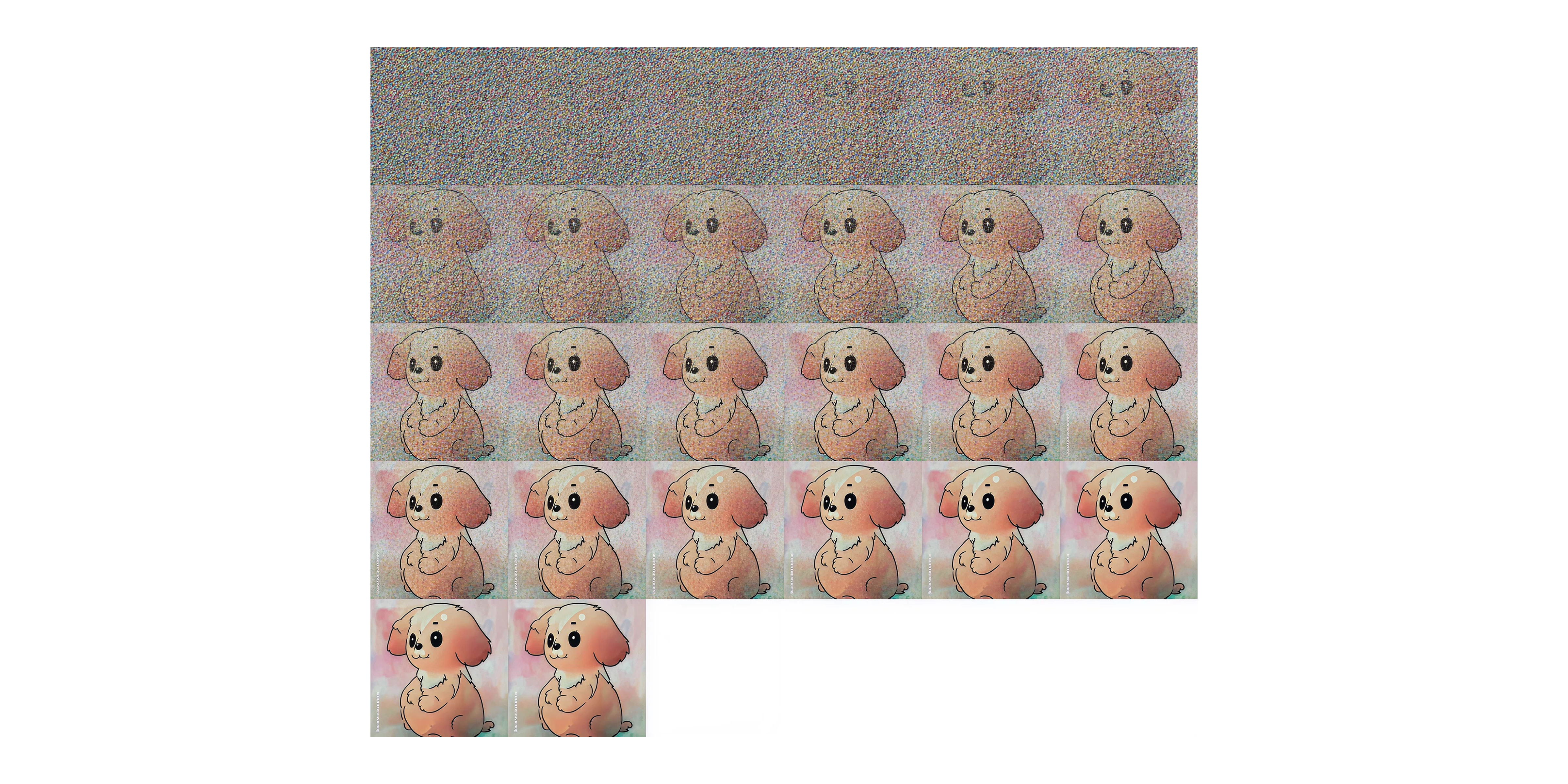
▲ Image progression across diffusion steps
The first thing we tried was reducing the amount of computation itself. More diffusion steps generally mean more refined images, but every step adds another round of computation. We ran a qualitative evaluation to see whether quality held up with fewer steps, and found that going from 50 steps to 25 made no meaningful difference in output quality. We set the production default to 25 steps, which cut compute roughly in half.
Stage 2. Parallelizing with Ulysses Sequence Parallelism (USP)
Alongside cutting computation, we also applied a parallelization strategy by adding GPUs and splitting the work across them. There are several ways to parallelize: Tensor Parallelism (TP), Sequence Parallelism (SP), Pipeline Parallelism (PP), and others.
For something like the Vision Decoder, which has to process a long fixed sequence of around 9K tokens, SP, which splits the input sequence across the available GPUs—fits well. Instead of one GPU handling all 9,000 tokens, several GPUs split them up. Within SP, we wanted to minimize communication overhead, so we went with Ulysses Sequence Parallelism (USP).
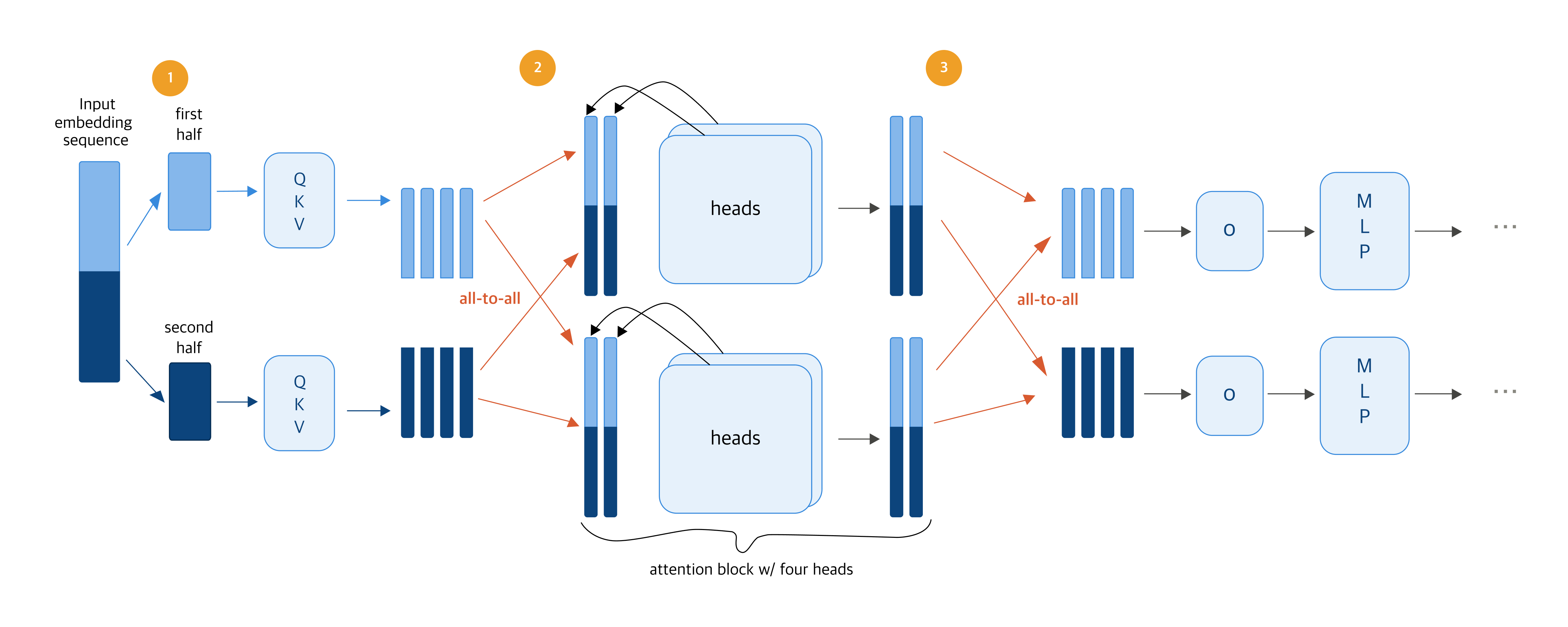
▲ “Ulysses: Unlocking Low-Latency, High-Throughput Inference for Long-Context LLMs”
Source: Snowflake Engineering Blog
The diagram above shows how USP works. Let’s walk through it with two GPUs.
1) Sequence splitting: Each GPU handles its own slice
Processing 9,000 vision tokens of image information on a single GPU is slow. So we split them across two GPUs—GPU 1 takes the first 4,500, GPU 2 takes the last 4,500—and each computes QKV on its own chunk in parallel.
- QKV: three vectors that capture what each token is, what it’s looking for, and what it can offer
2) All-to-all communication: Share the full context, then compute attention
Attention—the step that figures out how each token relates to every other—needs to see the relationships between all tokens. So at this step, just once, the GPUs exchange all their QKV information. That’s called all-to-all communication. After that, each GPU analyzes the full content from a different angle (attention head), with the heads computed in parallel.
3) All-to-all communication: Combine outputs, gather results, and finish
Once attention is done, the GPUs exchange results one more time (all-to-all communication) and gather the outputs (o) back into the token range each GPU originally owned. From there, the MLP step—which transforms each token independently—runs on each GPU with no further communication.
In this design, USP only needs to do all-to-all communication twice—before and after attention. As a result, even when you add more GPUs, the number of communication rounds stays the same, and the volume exchanged per round drops in proportion to the GPU count. That’s how USP keeps communication overhead minimal even on long sequences while still parallelizing efficiently.
In practice, we saw up to a 3.4x latency improvement on a 4-GPU setup. The image generation time that used to run on one GPU dropped to near the theoretical 4x ceiling—keeping the communication design simple let us turn nearly all of the added GPUs into actual speedup.
Performance optimization results
Through this series of optimizations, we saw meaningful latency improvements in each component: 3x from llm-d’s prefix-aware routing, around 4x for the Vision Encoder, and roughly 3.4x for the Vision Decoder.
This work was about more than just response speed. It built a serving foundation where performance, resource efficiency, and scalability can all be achieved together in a distributed inference environment. We’ll keep sharing what we learn from the problems we run into in production and the work we do to solve them.
Further reading
If you’d like to dig deeper into HyperCLOVA X 8B Omni serving, here are some resources to check out:
Model: HyperCLOVA X SEED 8B Omni on Hugging Face
Serving code: OmniServe GitHub repository
Paper: HyperCLOVA X 8B Omni (arXiv)
Previous post: HyperCLOVA X OMNI: Korea’s flagship AI on the road to omnimodality