
In this blog post, we introduce NAVER Cloud’s paper entitled “Peri-LN: Revisiting Normalization Layer in the Transformer Architecture,” which we presented at ICML 2025.
Why was large-scale LLM training more unstable with V100 GPUs?
V100 GPUs only supported FP16 (16-bit floating point) precision, which made large-scale model training inherently fragile. Even minor instabilities during training would cause loss spikes and NaN (not-a-number) divergence. Researchers at the time faced persistent concerns about potential failure.
Real-world evidence from the OPT logbook
According to Meta’s public OPT-175B training logbook, the team had to restart training 40 times in just the first nine days. With 1,024 GPUs in use, two or three would fail daily, and loss spikes and gradient explosions occurred repeatedly. Most of these issues stemmed from the combination of Pre-LN architecture and FP16 precision.
“We observed several catastrophic spikes and had to lower the learning rate to recover.” — OPT logbook
We’ll revisit the root causes of these problems later in this post.
Where can you find the normalization layer in the Transformer?
The Transformer architecture incorporates normalization layers to stabilize model training and information processing. Two widely adopted methods are LayerNorm and RMSNorm (Root Mean Square Layer Normalization), which we’ll refer to collectively as LN (normalization layer) throughout this post.
Most contemporary open-source LLMs employ Pre-LN structure as their default configuration. The placement of these normalization layers significantly impacts both training difficulty and stability.
- Post-LN was the original normalization strategy introduced with the Transformer architecture in 2017. It applies normalization to hidden states after computation, helping maintain model stability.
- Pre-LN represents the approach adopted by modern open-source LLMs including Llama, Qwen, Mistral, and DeepSeek. This strategy normalizes hidden states before each sub-layer computation, resulting in more stable training dynamics.
The emergence of Peri-LN
Past studies revealed that normalization layer placement significantly affects Transformer reliability and performance, leading to extensive research on Pre-LN and Post-LN architectures.
Recent major open-source models like Gemma2, Gemma3, and Olmo2, however, have begun adopting a different LN placement strategy. We term this previously unnamed structure “Peri-LN” in our research, as it places normalization layers peripherally around sub-modules. Our study analyzes its structural characteristics and performance advantages.
Peri-LN extends the existing Pre-LN architecture by adding normalization layers to module outputs, effectively normalizing both the input and output of each computation block. This architectural choice merits attention given its adoption by recent high-profile models including Gemma2, Gemma3, and Olmo2.
Normalization layers stabilize training by constraining signal variance. But what distinguishes Peri-LN from existing Pre-LN and Post-LN approaches? What motivated this design? We’ll examine these questions in the next section.
![]()
Figure 1. Placement of normalization in Transformer sub-layer
Hidden state variance
What are hidden states?
In Transformer architectures, each layer produces a d-dimensional vector known as a hidden state. As layers stack progressively deeper, these vectors accumulate the contextual and semantic information necessary for the model’s understanding and processing capabilities.
The critical factor here is hidden state variance. When this variance grows too rapidly, model training becomes prone to instability during the training process. Conversely, when variance is properly regulated, training proceeds stably through completion. The rate of variance growth serves as a key indicator of training success.
We’ll analyze the three normalization strategies from two perspectives: initialization and training.
Initialization phase: “Before starting the engine”
The initialization stage refers to the pre-training phase when model parameters contain only random values. At this stage, the variance patterns for the three normalization structures are:
- Post-LN: Variance remains approximately constant.
- Pre-LN: Variance increases linearly, though actual training dynamics prove more complex.
- Peri-LN: Variance increases linearly, similar to Pre-LN.
Most existing research has concentrated on this initialization phase through static analysis, which explains why Pre-LN and Peri-LN appeared functionally equivalent. However, recent discoveries of massive activations in fully trained models have highlighted the necessity of examining the complete training trajectory. (Read the referenced paper.)
What occurs between the initialization stage and training completion? Static analysis of initial conditions misses the dynamic phenomena that emerge during training. For reliable real-world training, analyzing initial values alone proves insufficient—we must track the dynamic changes throughout the entire training process.
Training phase: “Fueling the engine and stepping on the pedal”
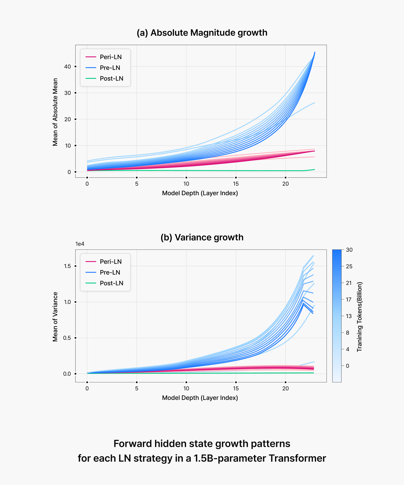
Figure 2. Forward hidden state growth patterns for each LN strategy in a 1.5B-parameter Transformer
When training commences, random parameters get gradually updated. Just like when you put fuel in your car and step on the accelerator, this is when actual changes begin to occur. At this point, significant differences emerge in hidden state variance and gradient flow depending on the normalization structure:
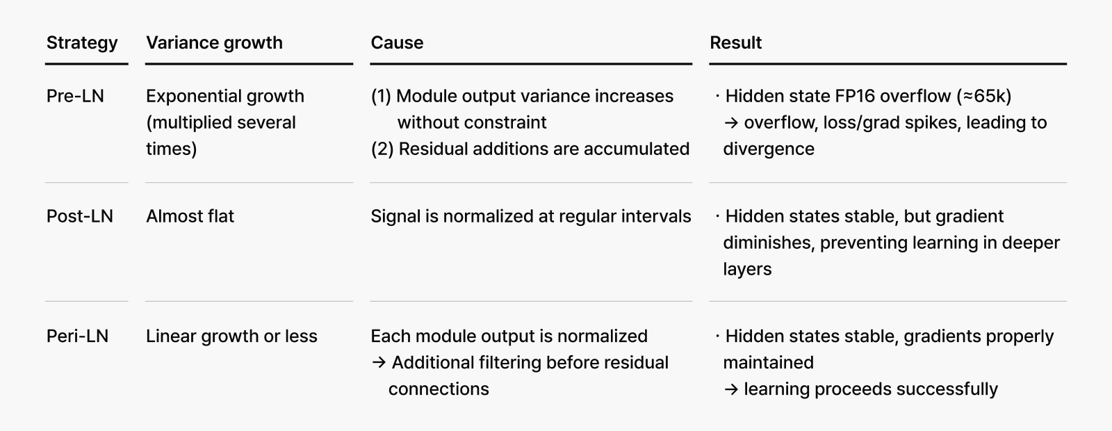
- Pre-LN: The initially linear variance growth becomes exponential early in training, leading to the phenomenon known as “massive activations.”
- Post-LN: While variance remains controlled, gradients diminish and fail to propagate effectively to deeper layers, essentially excluding lower layers from training.
- Peri-LN: Maintains equilibrium between variance control and gradient flow, mitigating both problems.
💡 Tip. When hidden state variance becomes excessively large, the optimizer loses directional guidance because noise overwhelms the signal. This impairs the model’s ability to determine what to learn and how much to learn, potentially causing loss spikes, gradient explosions, or complete training divergence.
Peri-LN is specifically designed to mitigate these dangerous instabilities.
The mathematical foundation
Why do these differences occur?
- Pre-LN creates a bidirectional loop where hidden vector magnitude grows with each layer.
- Peri-LN applies additional normalization to outputs, breaking this loop.
This explains why Peri-LN maintains controlled variance growth and stable training even with identical learning rates and weight updates.
1. Pre-LN
In Pre-LN architecture, the following relationship holds:
![]()
Here, k is defined as:
![]()
Therefore, input variance multiplies by (1 + k), and when 1 + k > 1, variance grows exponentially.
2. Peri-LN
Peri-LN architecture follows a different formulation:
![]()
Here, β₀ maintains constant-level variance, resulting in linear variance growth.
Pre-LN creates an amplification loop where larger inputs produce proportionally larger outputs, creating a risk of runaway variance growth as training progresses. Peri-LN breaks this loop by applying an additional normalization to the module output. Consequently, even with identical learning rates and weight updates, Peri-LN maintains controlled variance trajectories that scale linearly, ensuring stable training throughout the entire process.
Does large variance lead to training instability?
Large variance alone doesn’t necessarily cause training failure. The real problem is that variance and gradient magnitude are coupled through a multiplicative relationship.
In Pre-LN structures, gradient norm scales proportionally with hidden state norm, meaning that variance growth directly amplifies gradient magnitude, potentially leading to training instability.
Peri-LN addresses this by applying normalization layers after each attention and MLP module, effectively decoupling this multiplicative relationship. This prevents gradient explosion even when variance is large, maintaining training stability.
Examining hidden state variance in Pre-LN structure
A simplified Pre-LN layer can be expressed as:
![]()
When module output variance increases, xl + 1 grows proportionally. In our analysis, this relationship is:
![]()
When k > 0, variance continues multiplying and grows exponentially. The critical problem is that gradient magnitude is directly proportional to hidden state magnitude:
![]()
⇒ As hidden vector ||h|| increases, gradient explosion occurs!
What if we add a spoon of Peri‑LN? 🪄
Peri-LN applies normalization twice—before and after each module.
![]()
By applying an additional normalization layer to the module output, the output variance is constrained to near-constant levels β₀, resulting in linear (or sub-linear) variance growth:
![]()
Gradient magnitude is also automatically stabilized, as the final output hidden state ||a|| appears in the denominator, providing natural damping:
![]()
Training stability
As shown in the figure below, Pre-LN structures exhibit clear instability during large-scale LLM pretraining. Loss spikes and gradient explosions are commonly observed, with training divergence occurring in severe cases. In contrast, Peri-LN structures show no signs of instability under identical conditions and maintain significantly more stable training trajectories throughout the process.
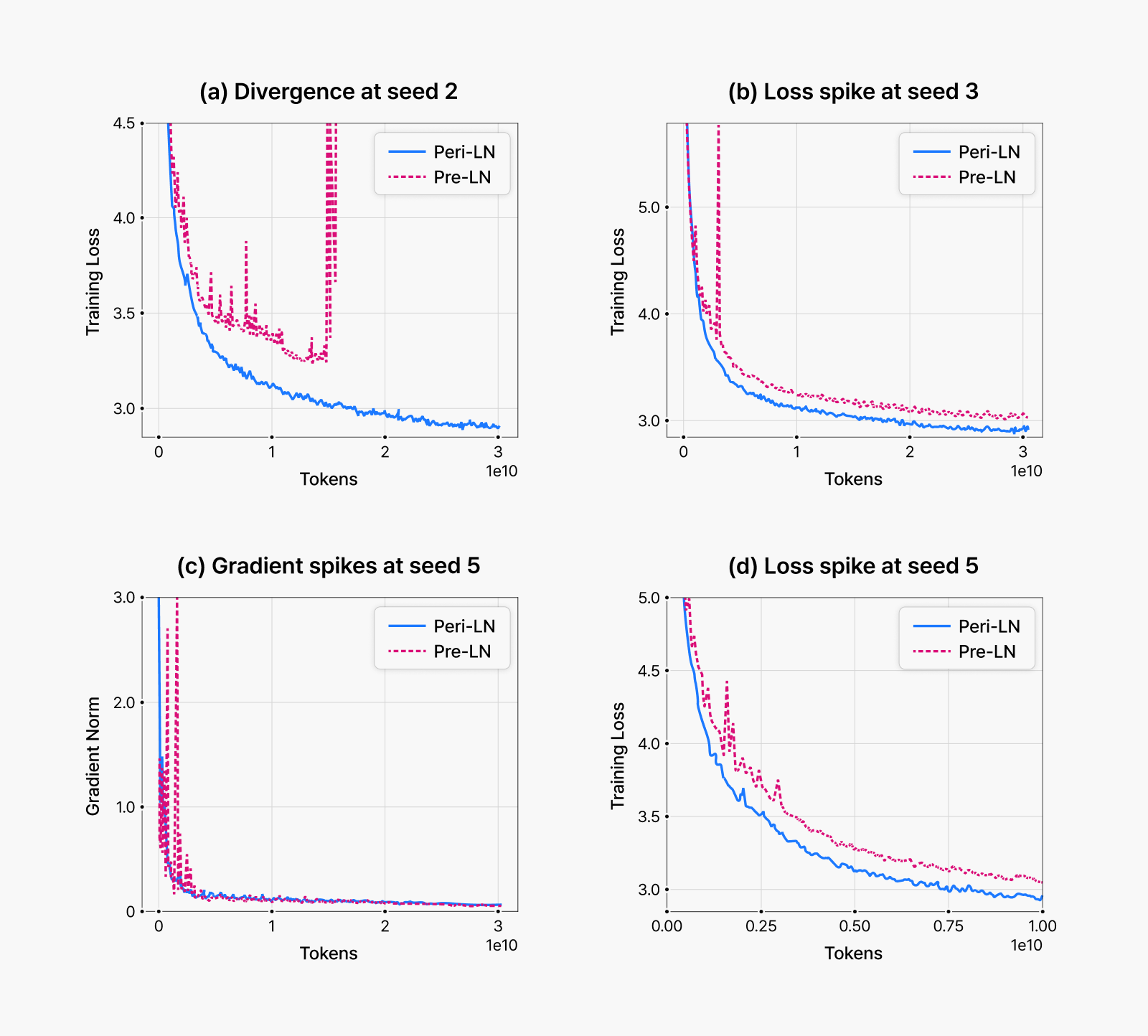
Figure 3. Common instability patterns during early-stage pretraining. Across multiple experiments with different random seeds, Pre-LN architecture consistently exhibited early-stage instabilities. While we initially suspected high learning rates as the primary cause, reducing them did not substantially resolve these issues. Under identical settings, Peri-LN demonstrated stable training curves. Panels (a), (b), and (c) show results from 400-million-parameter models, while (d) presents results from a 1.5-billion-parameter model.
Does massive activation really cause training instability?
Weight decay is a normalization technique that maintains parameter magnitudes at consistent levels during training and is known to be closely related to training stability. (Read the referenced paper.)
As shown in panel (a) of the figure below, applying weight decay can suppress massive activations. In Pre-LN architectures specifically, we successfully eliminated massive activations by applying substantially large weight decay coefficients.
These experimental results directly support our earlier conclusion that large hidden states cause gradient instability. To validate this relationship more definitively, we conducted additional experiments to determine whether massive activations actually cause training instability. Our methodology was as follows: we replicated training configurations that previously resulted in divergence, then applied strong weight decay to suppress massive activations and observed whether training stabilized.
Panel (b) demonstrates that once massive activations were eliminated, training proceeded stably. Through these experiments, we established that excessively large hidden states (massive activations) directly cause gradient instability.
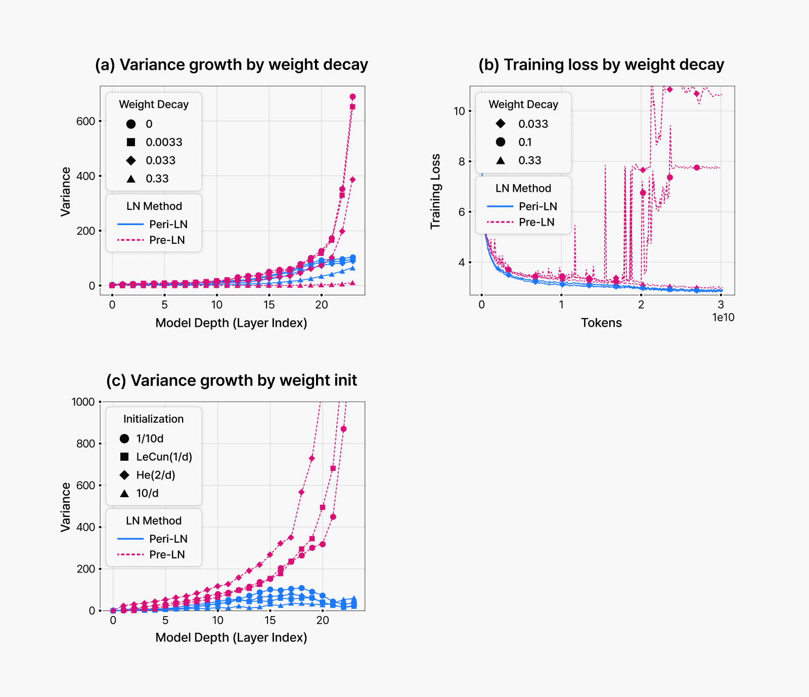
Figure 4. Effects of weight decay and initialization on massive activations
Performance benchmarks by normalization layer architecture
Comparative evaluation of Transformer models using Post-LN, Pre-LN, and Peri-LN architectures across major benchmarks revealed that Peri-LN consistently achieved the most stable and superior performance. Across different model sizes and multiple training runs, Peri-LN demonstrated low variance and consistent results. This indicates that Peri-LN not only delivers the highest final performance but also provides the most reliable expected performance regardless of training conditions.
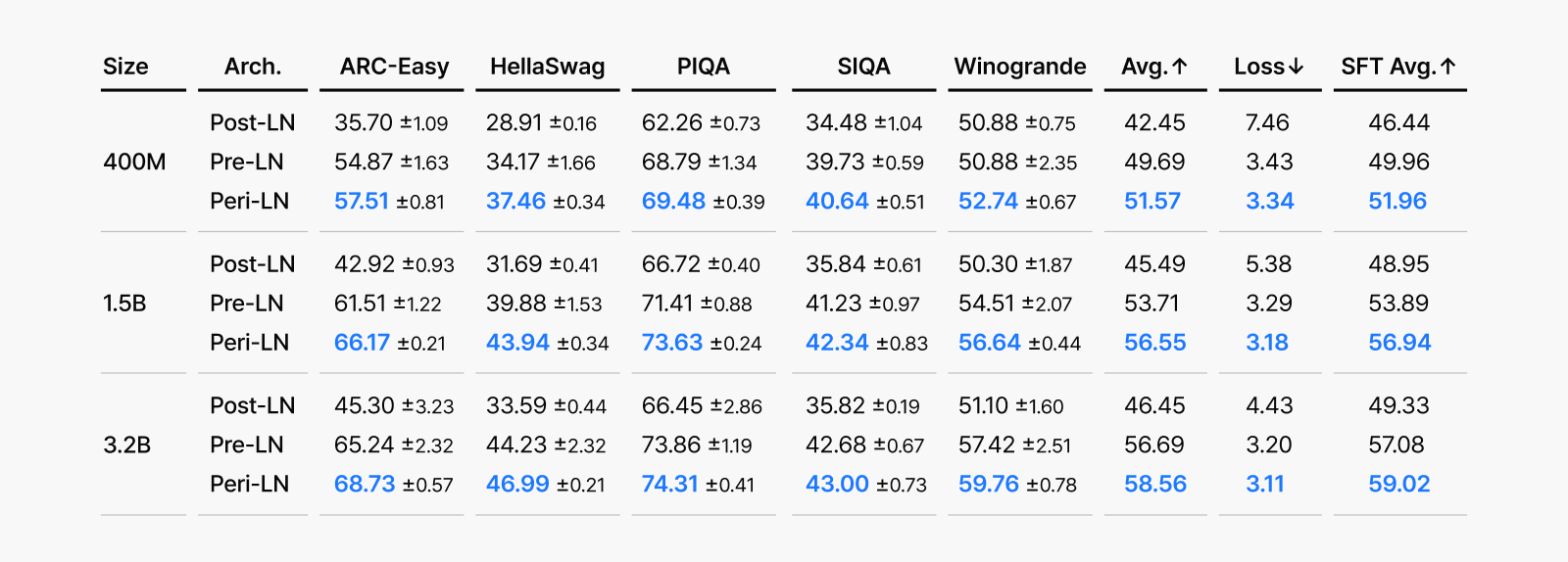 Figure 5. Comparison of LLM performance across various benchmarks when models with three normalization architectures (Post-LN, Pre-LN, and Peri-LN) are trained at different scales (400M, 1.5B, and 3.2B). Each score represents the average benchmark performance (with standard deviations) across 5 random training seeds.
Why is Pre-LN more dangerous in FP16?
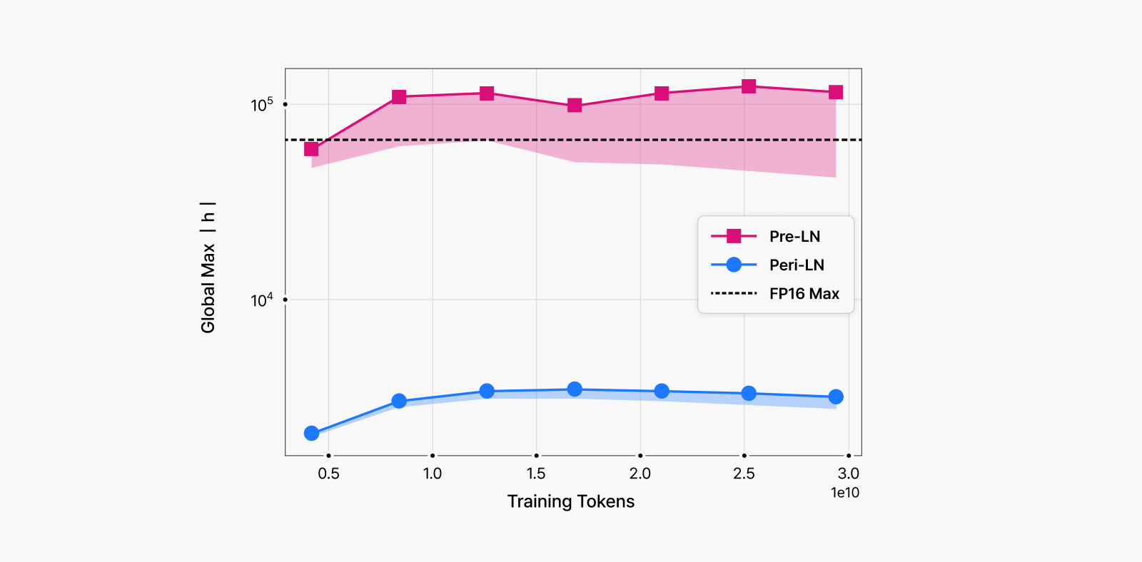 Figure 6. Graph observing how high hidden state absolute magnitudes can go during training
The colored bands in the graph trace the range of the top 100 absolute activation values.
- Pre-LN (red) increases rapidly as training progresses, surpassing the maximum value representable in FP16 format (orange dashed line).
- Peri-LN (blue) remains well below this threshold throughout the entire training process, maintaining numerical stability.
This graph demonstrates that Peri-LN effectively prevents massive activations.
Let’s return to our original question: Why was large-scale LLM training more unstable with V100 GPUs?
As explained earlier, Pre-LN architectures generate progressively larger hidden states in deeper layers as model size increases. When these values accumulate without normalization, particularly in models of 3B parameters or larger, they easily exceed FP16 limits (Figure 6). Such extreme hidden states lead to loss spikes, divergence, and other severe training instability—phenomena that have been extensively documented in actual OPT training logs.
While the BF16 format supported by A100+ GPUs has largely mitigated this issue, the same instability problems persist when using FP16 format. Consequently, FP16 environments experience stability gaps during both training and inference, resulting in measurable performance differences between FP16 and BF16 in practical applications.
Conclusion
This research analyzed the novel Peri-LN Transformer architecture and examined the underlying causes of training instability in Pre-LN structures. Scaling models safely is as crucial as scaling them larger. Peri-LN provides an additional layer of protection, enabling stable training of large language models even at scale. If you are concerned about LLM training instability, adopting the Peri-LN architecture could be a solution.
Our research journey reinforced that service and research are not independent parallel tracks. Real-world challenges we encountered—training instability—directly informed our research questions. The insights we developed through research were then integrated back into production systems, improving service performance. When we address practical problems through theoretical frameworks, the “why” becomes clear; when we apply validated theories to products, we accelerate the “how.”
We believe this research-production bridge represents an essential safeguard for the large-scale LLM ecosystem. Moving forward, we will continue transforming service challenges into research opportunities while translating research findings back into product improvements, strengthening the connection between the two domains.
For comprehensive details, see our complete paper: “Peri-LN: Revisiting Normalization Layer in the Transformer Architecture” presented at ICML 2025.