
Beyond building infrastructure: Why efficiency matters
Developing sovereign AI means taking on enormous costs. According to the model card Meta published in 2025, pretraining Llama 4 consumed a cumulative 7.38 million H100 GPU hours. Converted at current 2026 cloud rental rates for H100s (roughly $2.5–3 per hour), that comes to $18.5–22 million in GPU costs alone, or 25–30 billion Korean won. In an era where simply running GPUs for millions of hours costs tens of billions of won, a 1% gain isn’t just a technical win—it’s hundreds of millions of won. Building top-spec infrastructure matters, but so does the engineering skill to use that infrastructure without waste—a key competitive advantage in TEAM NAVER’s sovereign AI work. The pretraining scale of recently released multimodal models shows just how much is at stake.
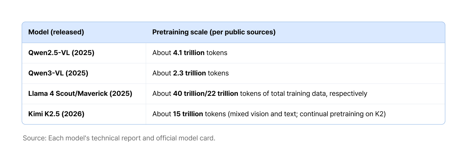
Source: Each model’s technical report and official model card.
TEAM NAVER runs large-scale LLM training infrastructure on its own clusters. But when we trained multimodal models, scaling up hit an unexpected bottleneck. Training speed that had been excellent on smaller models stopped improving as we expected once we grew both the model and the cluster. The infrastructure was top of the line, so why couldn’t we get its full performance in practice?
The cause: compute load imbalance across GPUs. When one GPU falls behind, the other thousands sit idle waiting for it—the “straggler” problem—and that translates directly into enormous wasted spend.
NAVER Cloud has been working with NVIDIA to solve these problems at the framework level. Parallelization strategies for large-scale training frameworks have evolved mainly around text-only LLMs, which is why optimization for a newer workload like packed multimodal sequences is still an active area of research today. Training HyperCLOVA X multimodal models on Megatron Bridge, NVIDIA’s open-source training framework, showed us where our own pipeline had room to improve. As a result, we raised training throughput by 50.2% on a 30B MoE multimodal model, and we’ve contributed the fixes back to Megatron Bridge. For the full technical detail on all four optimization areas, see the NVIDIA developer blog.
The packing and redistribution work—our fix for image token imbalance—contributed a 13.3% throughput gain on its own. Here’s how we found this invisible bottleneck and solved it without trading away model quality.
Multimodal pretraining: Changing the order doesn’t change the result
A multimodal model—in particular a vision-language model (VLM), which connects sight and language—is built from two main modules. First, the LLM, which handles the model’s “thinking.” Because it serves as the central pillar of VLMs and of omnimodal models more broadly, the LLM is also called the backbone—and TEAM NAVER’s was the first open-source LLM in Korea. Second, the vision encoder, the model’s “eyes.” We built our own for this: HyperCLOVA X CLIP.
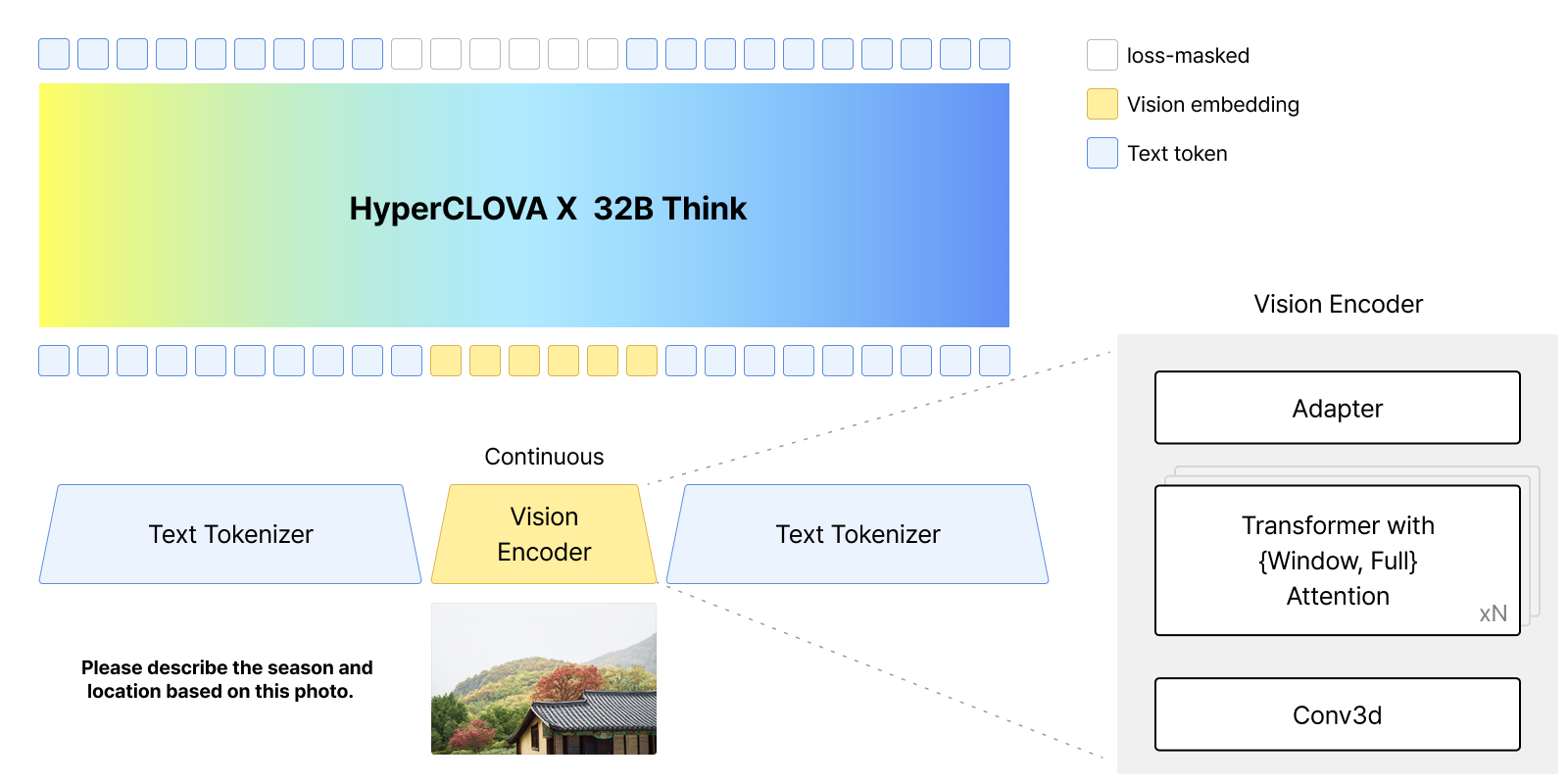
Figure 1. The structure of a VLM (excerpted from the HyperCLOVA X technical report).
Images pass through the vision encoder to become image tokens and text passes through
the tokenizer to become text tokens; both then enter the LLM as a single sequence.
When a sample containing both images and text comes in, the images pass through the vision encoder to become image embeddings, and the text is tokenized into text embeddings. The tokens corresponding to image patches are called “image tokens,” and those corresponding to text are “text tokens.” Everything that follows rests on one fact: the LLM’s compute load is determined by the sum of the two—the total token count—while the vision encoder’s compute load tracks the image token count alone.
Training AI models at scale relies on data parallelism. The training data is split into thousands of shards, thousands of GPUs compute on them at the same time, and the results each one produces—gradients—are summed so that every GPU updates the model with identical values. That summation is called all-reduce, and it doubles as a synchronization point, since it can’t finish until every GPU has joined. In multimodal training especially, the data that has to be read is far larger than in text-only training, so we design each GPU to read its assigned shard contiguously. Reading consecutive files without duplicate reads speeds up I/O, but as we’ll see, the design carries one implication: which GPU ends up with image-heavy data is purely a matter of luck.
On top of that comes gradient accumulation. When GPU memory limits how much data can be processed at once, the global batch is divided into several smaller micro-batches computed in sequence; the gradients from each step accumulate, and once a set number have piled up, the model weights are updated all at once. It’s a bit like scanning a large picture in pieces because no scanner is big enough for the whole thing, then stitching the scans together. The processing happened in pieces, but the result is identical to scanning the original in one pass.
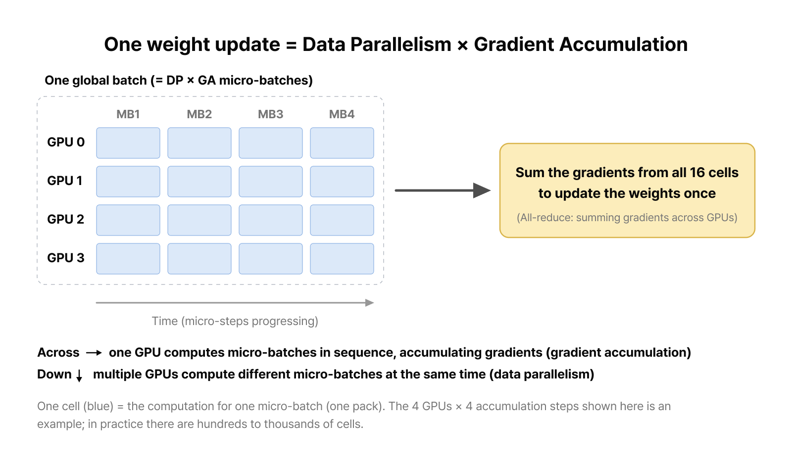
Figure 2. A single weight update consists of GPU count (DP) × accumulation count (GA) micro-batches, and the gradients from every cell are summed and applied at once.
There’s one thing to take away from Figure 2: the computation behind a single update is ultimately just summing the gradients from every cell, and addition gives the same result no matter what order you do it in.
Bottlenecks in multimodal training show up in several places—data I/O, vision encoder compute efficiency, and more—but this post focuses on the one that was hardest to find and hardest to optimize: compute load imbalance across GPUs.
1. Sequence packing: Filling the box with no gaps
Before getting into the imbalance itself, let’s cover why we use packing to optimize LLM backbone training. Packing is the process of fitting training data of wildly varying lengths into fixed-size “boxes”—fixed-length sequences—with no gaps, turning them into units of work for the GPU. It’s like pressing odd-sized items into a suitcase to squeeze out the empty space. So why go to the trouble of filling them this tightly?
Because in training very large models, most of the compute happens in the LLM backbone. What drives training cost is how little the LLM wastes on empty data, which makes sequence packing—minimizing empty space to raise data density—the most basic and also one of the most powerful optimizations available.
The problem is that training data comes in all different lengths. Sample lengths—the length of a single training example—can differ by more than an order of magnitude, yet training requires them all to be the same length. Filling out a short sample to that fixed length with empty space, or padding, wastes a lot of compute. In the example in Figure 3 below, gathering samples ranging from 1,200 to 4,200 tokens into one batch pushes the padding ratio to roughly 40%—40% of the box is being shipped full of air. The usual approach in LLM training, “streaming” (concatenating samples and cutting them at the sequence length), creates a different problem: images get sliced at sequence boundaries. Text can be cut mid-stream, but an image is a single unit and can’t be split down the middle.
So in every experiment we use greedy bin-packing, which fills a fixed-length sequence with whole samples to minimize padding. Because packing operates on whole samples, images never get cut at a boundary, and at an 8K sequence length we reach a packing efficiency—the share of total tokens occupied by real data—of 99.4%.
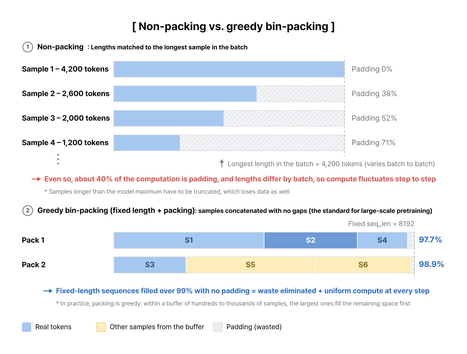
Figure 3. Padding to the longest sample in the batch still wastes a substantial amount when sample lengths vary, and the compute per batch fluctuates (top). Applying greedy packing to fixed-length sequences fills more than 99% with real data and makes the compute uniform (bottom).
Back when we trained on text alone, this was enough. If every GPU’s sequence was full at the same length, the compute was the same and so was the time it took, so nobody had to wait.
2. Same box, different weight: The problem images introduced
Once models started training on images too, an imbalance in vision encoder compute began to show. As noted earlier, the LLM’s compute is set by the total sequence length—text plus image—so identical pack lengths mean identical work for every GPU. The vision encoder’s compute, though, tracks the number of image tokens in the pack. A GPU that draws an image-heavy pack spends proportionally longer in the vision encoder.
This is where packing’s blind spot shows up. Greedy packing looks only at the total token count; it pays no attention to how many of those tokens are image tokens. The result is that one GPU’s pack is loaded with images (3,000 image tokens) while another’s is almost entirely text (500 image tokens). Two boxes of the same size: one packed with bricks (images), the other with cotton (text). Same volume, wildly different weight.
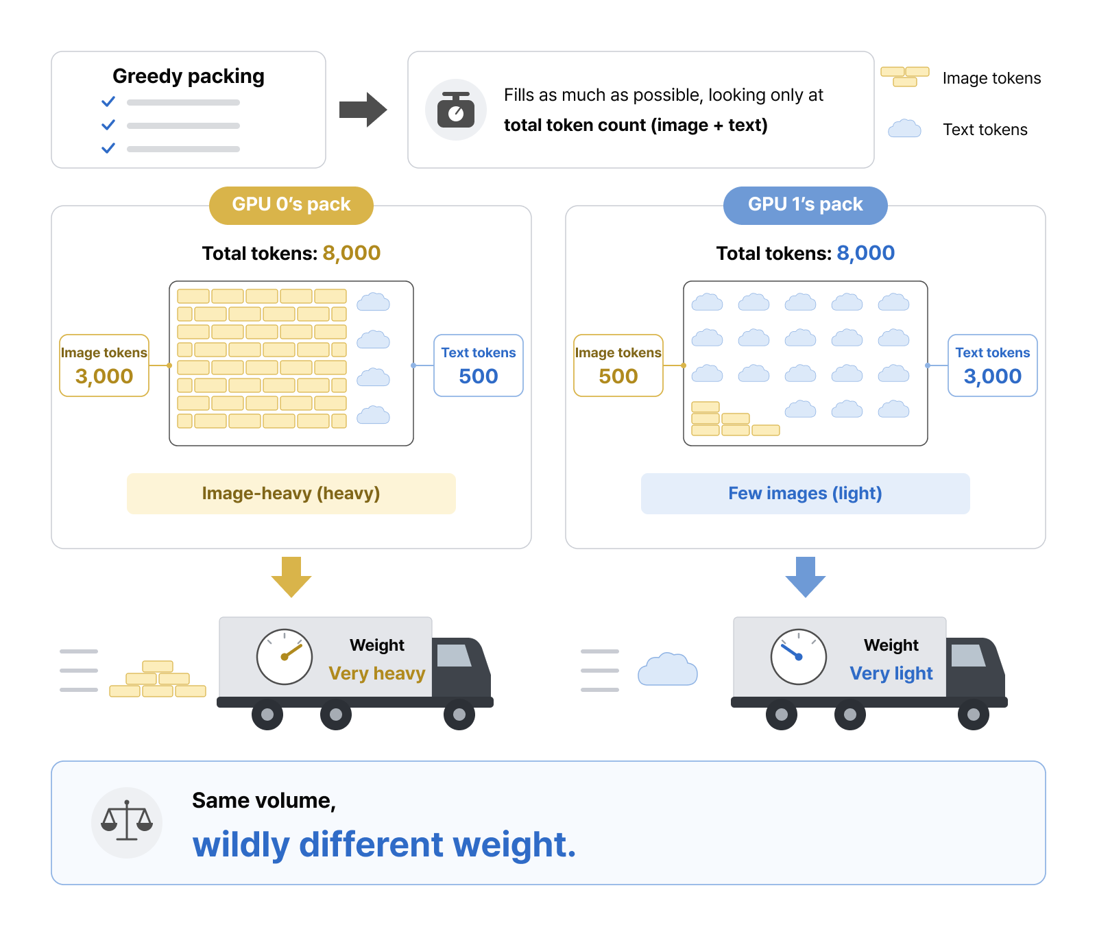
Figure 4. Both packs are full on token count, but one holds six times as many image tokens as the other.
Both packs are exactly 8,192 tokens long, but the compute they demand is nothing alike. In our measurements, the GPU handling the 3,000-image-token pack spent 900 ms on the vision encoder forward pass alone; the GPU with the 500-token pack spent 200 ms. That’s a 700 ms gap right out of the gate—and the gap widens once more. A single training step runs vision encoder forward → LLM forward → LLM backward → vision encoder backward, and the gradient synchronization barrier, where all GPUs come together to reconcile their results, sits at the very end. The LLM stretch is identical for both GPUs because the lengths match, but a backward pass typically costs about twice as much as a forward pass, so the Vision Encoder backward opens the same proportional gap a second time. The GPU that reaches the barrier first has no choice but to sit idle for the full accumulated gap, waiting for the slowest GPU to arrive.
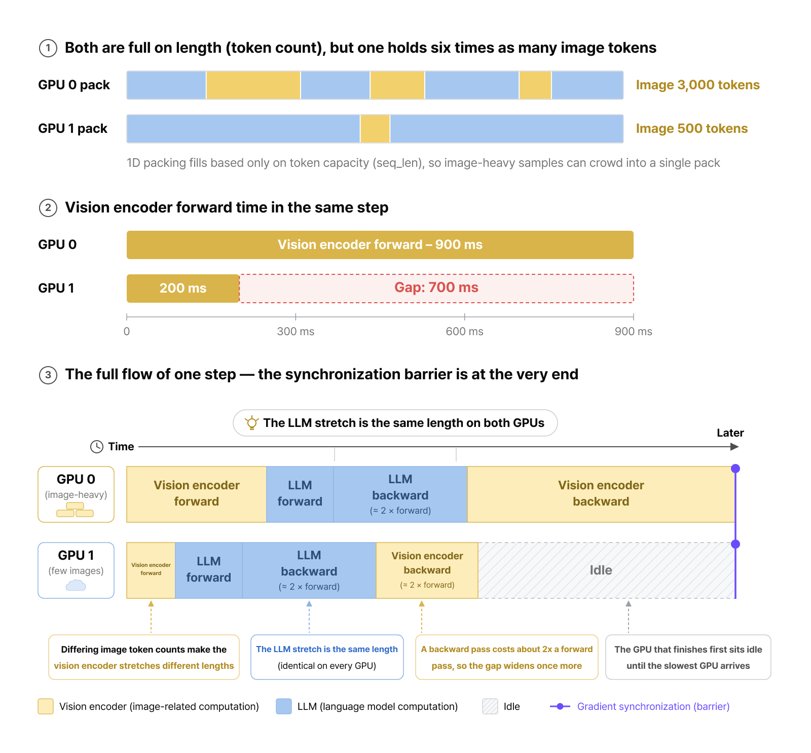
Figure 5. The vision encoder forward pass alone opens a 700 ms gap (top). The synchronization barrier sits at the very end of the step, after the LLM forward and backward passes and the vision encoder backward pass have all finished; because the backward pass widens the gap by the same proportion, the actual wait is longer than this (bottom).
With two GPUs it’s manageable. With 1,024 training together, the single card that draws the heaviest pack sets the pace for all of them—and the more GPUs there are, the higher the odds that at least one ends up with a very heavy pack. Simulations built on measured data showed the same trend clearly: time wasted waiting on slow GPUs climbed from 50% to nearly 80% of total training time as LLM model size and GPU count grew. In text-only pretraining, compute imbalance barely surfaced. In multimodal training, it’s the thing that blocks scaling.
3. First attempt: Adding “weight” to a box that only tracked volume (2D packing)
Each GPU—more precisely, each data parallel worker holding its share of the data—can only see the data assigned to it. The first solution that comes to mind is to check the image token count alongside the total token count during each worker’s own packing step. Put simply: when filling the box, look at weight as well as volume.
If conventional greedy packing is 1D packing—filling along the single axis of “token length”—then 2D packing adds a second axis: “image volume.” The method is simple. Each pack gets an image token “budget,” and once the budget is exceeded, image-heavy samples no longer go into that pack. If it worked, we’d resolve the imbalance without workers having to exchange any data at all. To find out, we simulated several approaches using measured values for the total length and image token count of our actual training data.
But the approach had a serious problem: it couldn’t fill the sequence. Excluding image-heavy samples over and over left empty space behind, and packing efficiency crashed from 99% to 66%. Training with 34% of the token capacity sitting empty every step defeats the whole purpose of packing, which was introduced to eliminate wasted padding in the first place.
Would a larger pool of candidates help—say, thousands of samples in the packing buffer? It didn’t make the problem go away. Each pack still runs out of image budget while token space remains. Filling that leftover space requires samples with almost no images, and since most multimodal training data contains images, no amount of extra candidates produced enough samples that fit.
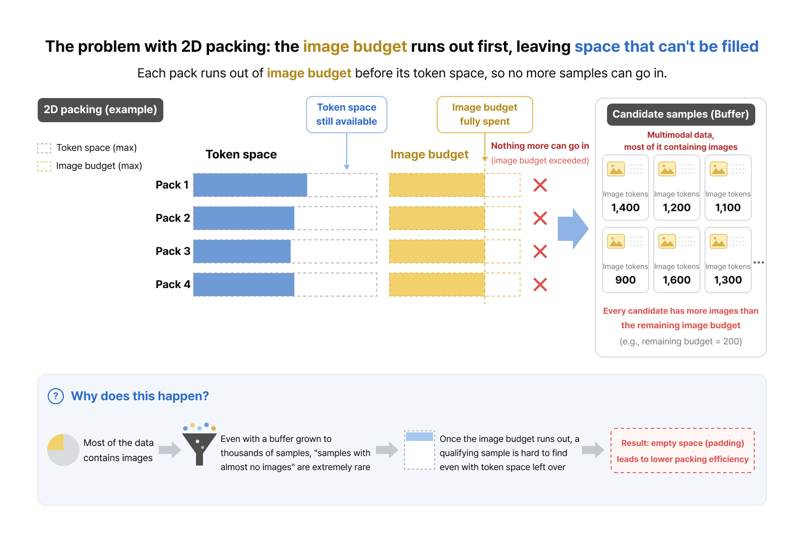
Figure 6. Adding an image budget balances image tokens across packs, but the image budget runs out before the token space does, dropping packing efficiency to 66%. Growing the buffer to thousands of samples doesn’t fix it, because there aren’t enough image-free samples to fill the leftover space.
What about simply making the image budget generous? A larger budget brings packing efficiency back to 99%, but image-heavy samples can crowd into a single pack again, and the imbalance returns with them. Push the budget to infinity and you land right back at the 1D greedy packing we started with. The image budget is just a dial between “well balanced but wasteful” and “densely packed but imbalanced,” and no setting satisfies both goals at once.
We simulated other variants too, including local reordering, where each GPU only changes the order in which it computes its own packs. They all shared the same limitation: each tries to solve the problem inside a single GPU’s own data. They helped early in training, then lost their effect as steps accumulated and balance drifted across GPUs—and the more GPUs involved, the faster they broke down.
The conclusion was clear. However you compose the box, however you reorder the computation, an approach confined to one GPU’s own data hits a ceiling. We had to widen the view to a placement problem “between” GPUs.
4. Don’t rebuild the boxes—have the GPUs swap them
The answer came from deep learning fundamentals. A deep learning model computes gradients over a batch of data, sums and averages the gradients from each example, then corrects the weights in a single pass. As Figure 2 showed, that computation is mathematically identical no matter what order you add in—or which GPU does the adding.
Which leads to the idea: there’s no need to redo the packing at all. Instead of each GPU rebuilding its boxes or shuffling their order, leave the boxes—already 99% full—exactly as they are, and have the GPUs simply swap boxes with each other right before computing. The goal is for heavy boxes (packs with many image tokens) and light ones (packs with few) to be spread evenly across the units of computation (the micro-batches) so that every GPU carries a comparable load at each micro-step.
Here’s how it works. For every global batch—one weight update’s worth of data—each GPU shares the image token counts of the packs it holds via an all-gather. Every GPU then computes the optimal placement using the same rule and exchanges packs micro-batch by micro-batch according to that result.
The placement is computed in two stages:
- Compute the optimal placement considering only compute balance, ignoring where each pack started out.
- Take the packs’ original locations into account and find a placement that achieves the same balance while minimizing how much data actually has to move. Packs already in the right place skip communication entirely.
The biggest advantage of this approach is that it doesn’t change the training outcome at all. The data doesn’t change, the model doesn’t change, the training results don’t change. The only thing that changes is “who computes what, and when.”
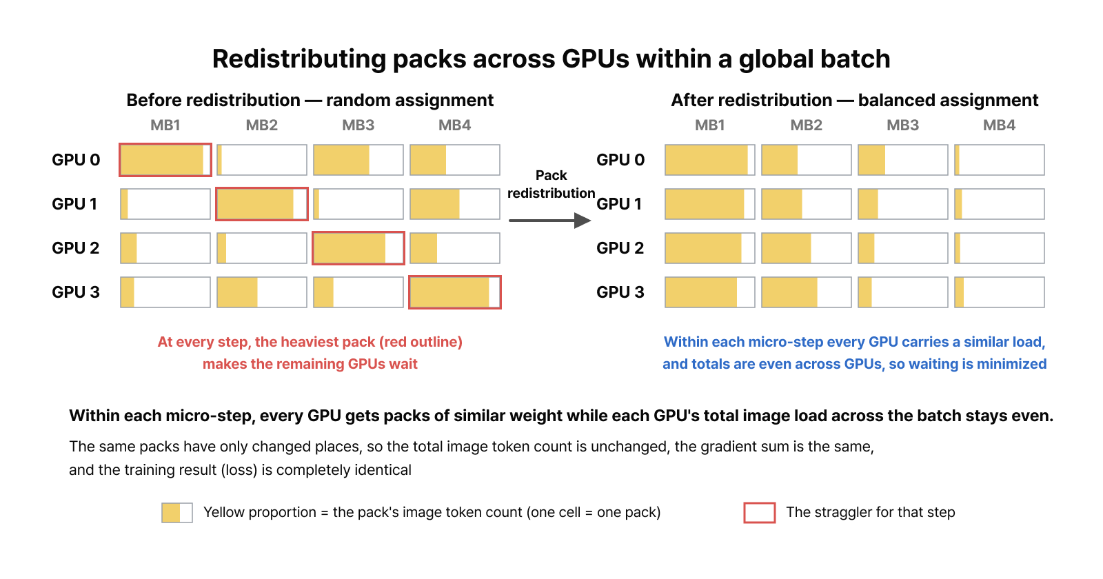
Figure 7. Packs being redistributed across GPUs within a single global batch. Within each micro-step, every GPU gets packs of similar weight—heavy ones scheduled alongside heavy ones—while each GPU’s total image load across the batch stays even. The computed result is mathematically identical; only the per-step waiting disappears.
5. Redistribution isn’t free: Hiding communication behind compute time (overlap)
Redistributing packs does come at a cost. The all-gather that shares image token counts is very light—a few integers per pack, kilobytes in total—but moving the pack data itself between GPUs, as the placement dictates, is far heavier. Handling that communication sequentially after each round of computation would hand back all the time we saved on straggler waits.
The fix is to hide that communication behind GPU compute time. While the GPU works through the forward and backward passes of the current micro-batch, a background thread and a separate CUDA stream redistribute the packs for the next micro-batch behind the scenes. By the time the GPU finishes computing, the balanced next pack has already arrived, so the cost of redistribution barely registers in training time. Overlapping computation and communication this way is called computation-communication overlap. It’s the same logic as prepping the next set of ingredients while the oven runs: total cooking time doesn’t grow by the length of the prep.
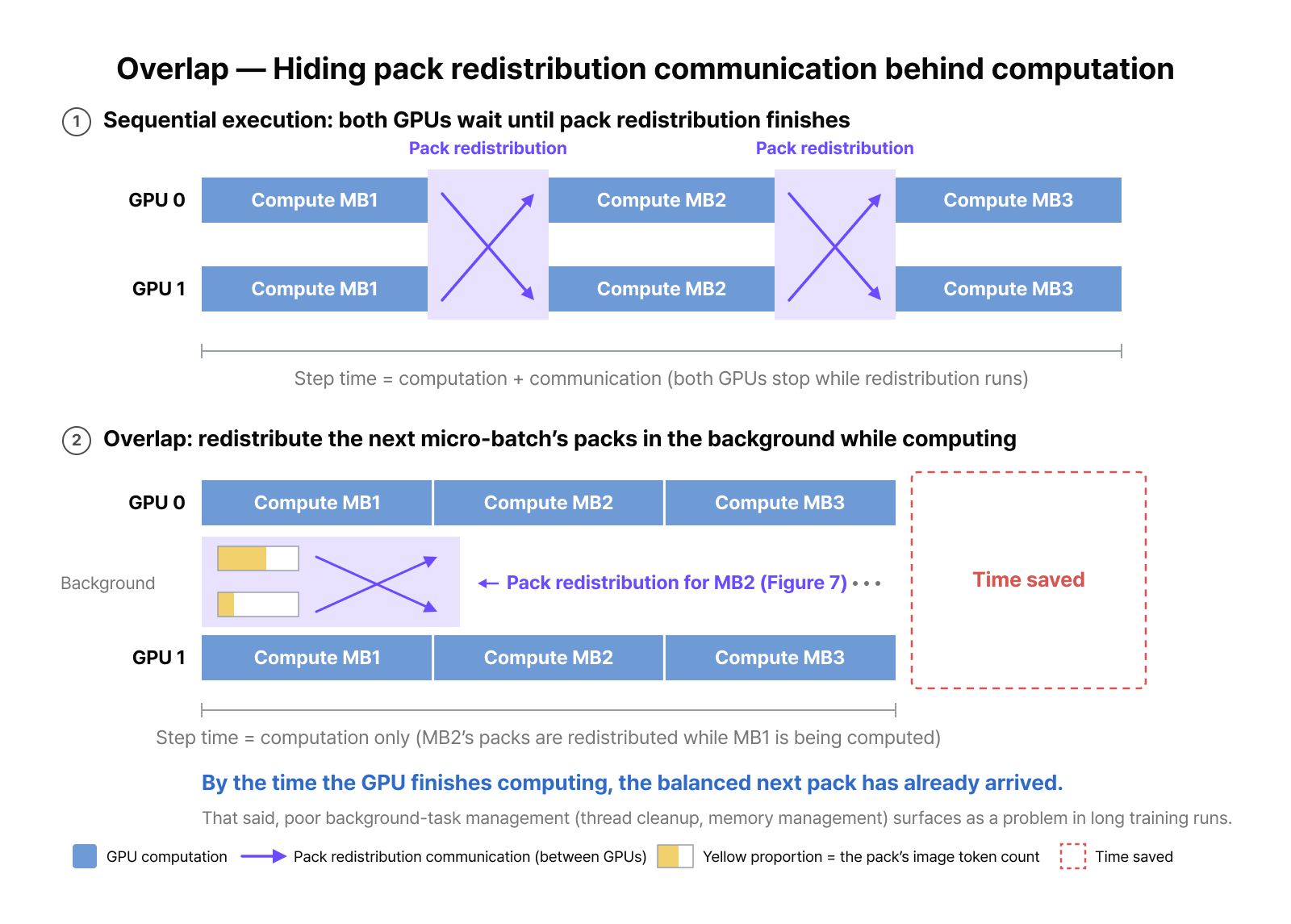
Figure 8. With sequential execution, every GPU waits until the pack redistribution
between GPUs finishes (top). With overlap applied, the pack redistribution for the next micro-batch (Figure 7) runs in the background while the current micro-batch is being computed,
so communication time disappears from the step time (bottom).
The numbers show how much overlap matters. In the production-scale experiment described below, running the redistribution synchronously—waiting for the communication to finish—yielded only a 1.7% improvement. Running the same redistribution asynchronously with overlap pushed that to 13.3%. The engineering that hides the cost mattered as much as the balancing algorithm itself, and it produced most of the gain.
A simple idea doesn’t mean a simple implementation, of course. We hit a memory leak where background threads weren’t joined after finishing their work, so resources piled up bit by bit. Bugs like this never surface in a short few-hundred-step benchmark; they show up as a gradual slowdown only in long runs past several thousand steps. Training speed stabilized only after a long stress test isolated the cause and we patched it. In training optimization, the idea is half the work—the other half is verification and debugging like this.
6. Results: Same training outcome, faster
We validated the final implementation, overlap included, in stages from small scale up to real production scale.
- Identical loss curves: that follows from changing only the computation order, but we confirmed it experimentally.
- Production-scale validation: with the data we actually use for pretraining (100-plus sources, more than 2 trillion tokens), a 30B MoE VLM, and a multi-node B200 environment, the packing and redistribution optimizations improved throughput—the amount of training processed in a given time—by 13.3%. Synchronous redistribution alone reached just 1.7%, so most of the gain came from overlap.
One caveat: as the LLM grows, the vision encoder accounts for a smaller share of total compute, so the size of the improvement shrinks. Even so, a double-digit gain is no small number in large-scale pretraining that consumes millions of GPU-hours. And it came without sacrificing an ounce of model quality.
Closing thoughts
Training optimization in the multimodal era asks a different question than it did in the text era. It’s not just how tightly you fill a sequence, but how the compute load gets shared across GPUs. The image token balancing described here is one of our answers to that question.
The packing and redistribution work covered here spans two of the four areas we optimized—sequence packing and distributed training, alongside storage I/O and the Vision Encoder. Together, all four improve training throughput by 50.2% on a 30B MoE VLM.
In training runs this expensive, knowing how to draw every bit of value out of the hardware matters more and more—and efficiency like this doesn’t end with a single improvement. The cost and time it saves get reinvested in larger models and a wider range of experiments, and that headroom raises the starting line for the next challenge. That’s what makes these optimizations more than a speed-up: they lay the groundwork for taking on bigger and more varied multimodal models on the same infrastructure. NAVER Cloud will keep sharing the problems we run into on real large-scale training runs and the insights we gain from solving them. We hope you’ll stay with us as our research and HyperCLOVA X continue to evolve.