
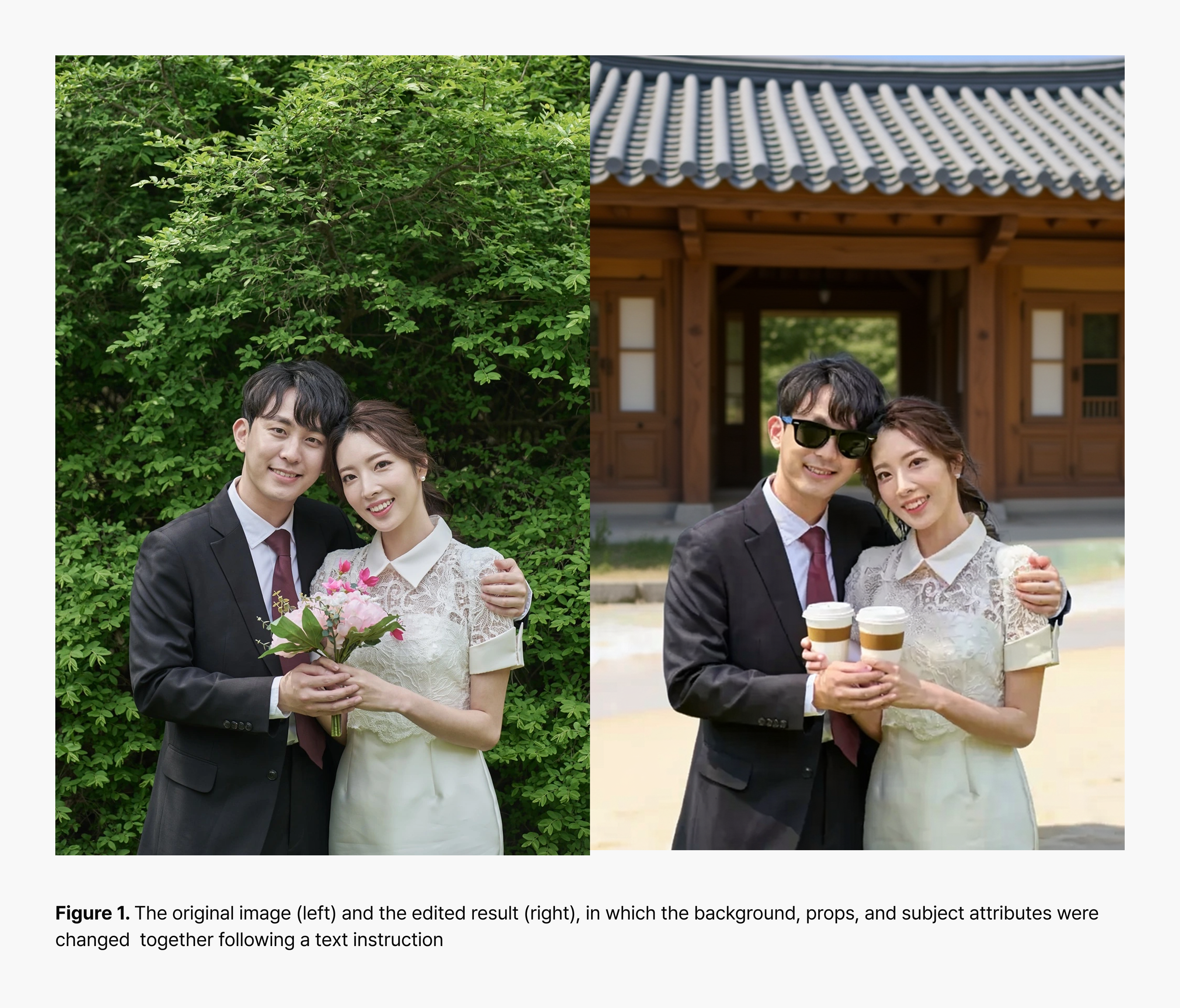
“Change the background to a hanok, a traditional Korean house, have both people hold coffee, and add sunglasses to the man.”
What does a model need to learn first to follow an instruction like this?
Image generation models are no longer just for making new images. They’re used across visual content production, including editing existing images to meet complex requests. That widening range asks more of a model: a wider variety of scenes to understand, and more complex instructions to handle.
That means training on more data and, when necessary, scaling the model up. But scale brings longer training times and heavier compute demands. The real problem is finding an architecture and a training method that can learn from enough data and reach the target quality within the available time and compute.
NAVER Cloud is training a large image generation and editing model from scratch, without pretrained weights. We wanted to design the architecture, the data, and the training objective together, track the entire training process, and keep improving the model on our own as service requirements change. Because we aren’t adapting an already-trained open model, we had to get generation right before the model could learn to edit.
There was a lot to decide: which latent space to compress images into, which backbone and optimizer to use, and which layers of the text encoder to draw text conditioning from—and how many of them. Even with the same data and compute, each of these changes how fast training converges and how good the output is.
We couldn’t just apply results reported in papers as is. The same technique can behave differently depending on model scale and architecture, data distribution, and what other techniques it is combined with.
So before committing to large-scale training, we validated promising techniques one at a time on small models. We then combined the techniques that showed clear benefits one by one, checking whether the gains held when they were used together. Here’s how we narrowed the candidates, what actually made a difference, and what we learned from the experiments that didn’t go as expected.
1. Finding answers in small models before the big training run
What mattered in the search for a training recipe wasn’t finding the single best score—it was keeping the experiment cycle short enough to move on to the next question quickly. We shrank model size and resolution so we could see each candidate’s trend within a few days, and took the simplest stable configuration as our baseline. From there we changed one element at a time so the cause of each result was clear.
The baseline was a Latent Diffusion Model (LDM) operating in a latent space compressed by a Variational Autoencoder (VAE). For the backbone that generates images, we used a Multimodal Diffusion Transformer (MMDiT).
Validation ran in two stages. First, in a class-conditioned generation experiment—where one of ImageNet’s 1,000 categories is given as the condition—we compared backbones, VAEs, training objectives, and optimizers, individually. That let us set aside the effects of interpreting a user instruction and look at the model’s own learning behavior. Techniques that showed promising results at this stage were further validated on text-to-image (T2I) data consisting of paired text and images. Because T2I was closer to our ultimate goal, we focused in particular on whether the gains from individual techniques held when they were combined.
For quantitative evaluation we used four metrics, each looking at a different aspect.
- FID [1]: How close the distribution of generated images is to that of real images. Lower is better.
- DINO-MMD [2, 3]: Compares the distributions of generated and real images in the representation space of the DINO visual encoder. Lower is better.
- CLIP score [4]: How well a generated image reflects the content of its caption. Higher is better.
- Aesthetic score [5]: An estimate of the aesthetic quality a person would prefer. Higher is better.
For differences the quantitative metrics miss, we compared by eye the images each model generated from the same prompts. To probe T2I weak spots that are hard to measure numerically—text, fingers, repeating patterns—we included prompts containing those elements.
When comparing architectures, we looked at wall-clock time alongside training steps. In large-scale training, the resource that actually runs out is GPU time, not step count. An architecture that learns more per step but takes longer per step ends up seeing less data in the same window.
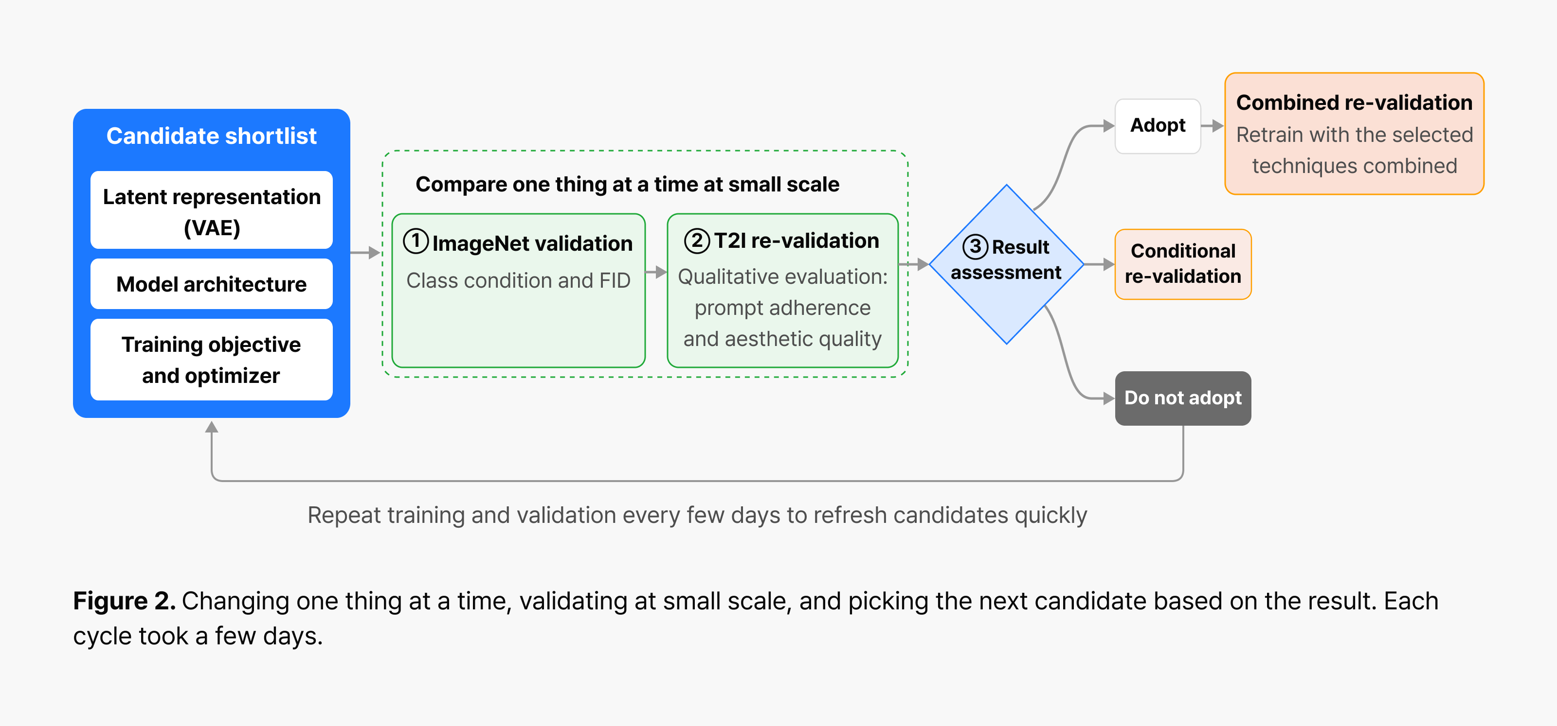
We didn’t sort the small experiments simply into adopted and dropped. We immediately adopted techniques with a clear difference even at small scale. Techniques that might only show their advantage as model capacity grows or input sequences get longer, we kept as candidates to revisit at larger scale.
2. Which techniques actually made a difference?
We started with which latent representation to use, how weights get updated, and which noise range to train on. To settle what would go into the final recipe, we then widened the scope to representation learning, information flow between blocks, and text conditioning.
Does the latent space change how fast a model learns?
Image generation models generally don’t train on every pixel of the original image. They first use a VAE to compress the image into a latent space the generation model can work with more easily, then learn the image generation process in that space. Turning the latent representation the model produces back into an actual image is also the VAE’s job.
Put simply, a VAE is a translator that converts an original image into a form the generation model can understand. Even with the same images, a different VAE means a different shape and distribution for the representations the generation model receives. So the choice of VAE can change both the difficulty and the speed of learning.
The same thing happens in an LLM: how a tokenizer splits input changes training difficulty. In image models, the properties of the latent space the VAE produces set the starting point for training.
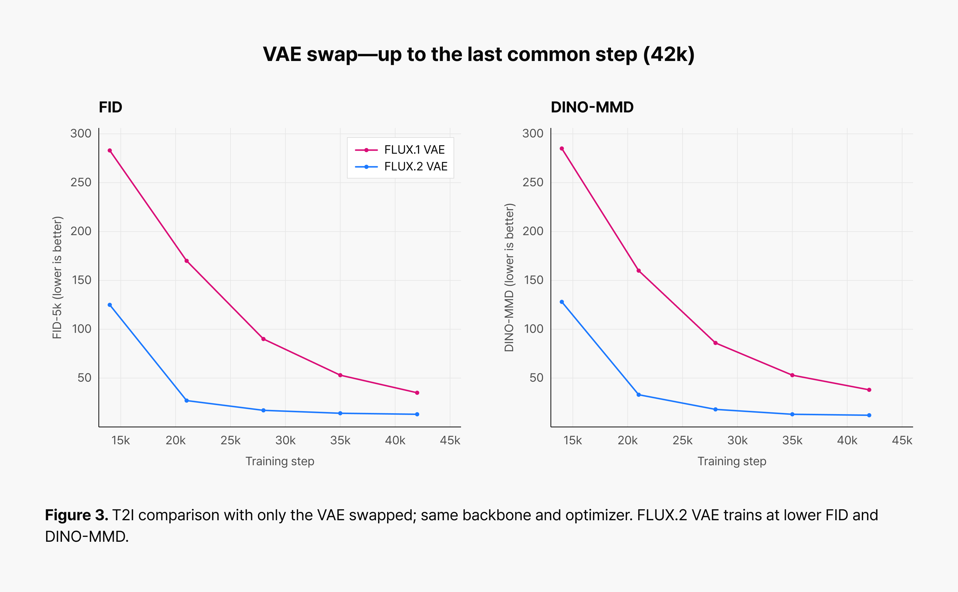
To examine this difference, we connected the FLUX.1 and FLUX.2 VAEs [6] to the same backbone and compared them. Throughput differed by only 0.4% between the two setups, indicating that their per-step training time was effectively comparable.
The training results clearly differed, though. At 225k steps, FID dropped about 7%, from 10.95 with the FLUX.1 VAE to 10.19 with the FLUX.2 VAE.
More striking than the final FID was how fast each setup reached the target quality. The point at which FID hit 30 moved from 87.5k steps to 50k steps—37.5k steps earlier for the model using the FLUX.2 VAE. Because throughput was nearly identical, those saved steps translated directly into saved training time.
That’s an important difference in large-scale training. A slightly better final score matters, but reaching the same quality in fewer steps and less time means more experiments on the same limited GPUs, or an earlier move to the next training stage.
This result reproduced the training-efficiency improvement reported for the FLUX.2 VAE in a similarly configured class-conditioned image generation experiment. Because our ultimate goal is text-guided image editing, we then tested whether the same trend held in a T2I setting with natural-language inputs.
At the last common step (42k), the FLUX.1 VAE baseline scored 35.12 on FID and 37.77 on DINO-MMD. Swapping in the FLUX.2 VAE brought those down to 13.19 and 11.05.
The gap appeared early in training in both the ImageNet and T2I experiments, leading us to conclude that the latent representation produced by the FLUX.2 VAE was better suited to training our model.
The graph below plots the stretch from 14k to 42k steps, where the two setups can be compared side by side.
How can a model learn more in the same number of hours?
Having settled the space the model would learn in, we turned to how its weights get updated in that space. An optimizer is the rule that turns the gradients computed during training into actual weight changes. Even with the same architecture and loss function, the optimizer can change how quickly the model reaches target performance.
We compared the widely used AdamW [7] with Muon [8]. Muon adjusts matrix-shaped weight updates so they don’t concentrate too heavily in particular directions. Because it leaves the architecture and loss function alone and changes only the update rule, it’s easy to compare directly against AdamW and combines well with other training techniques.
We started by comparing how many steps each needed to reach the same FID in the ImageNet experiment. AdamW reached FID 12 at 150k steps; Muon got there at 37.5k.
Muon does need extra computation to update weights, though, so its per-step time was longer than AdamW’s. Fewer steps alone isn’t enough to conclude that actual training time came down. To check, we compared the two setups again on wall-clock time. Thirty-six hours into training, FID was 10.19 for AdamW and 5.20 for Muon. Even accounting for the per-step overhead, Muon reached a lower FID in the same amount of time.
We also cut much of Muon’s extra computational load with a parallel implementation in our distributed setup. Since the quality gain held on wall-clock time as well as step count, Muon went into the final training recipe.
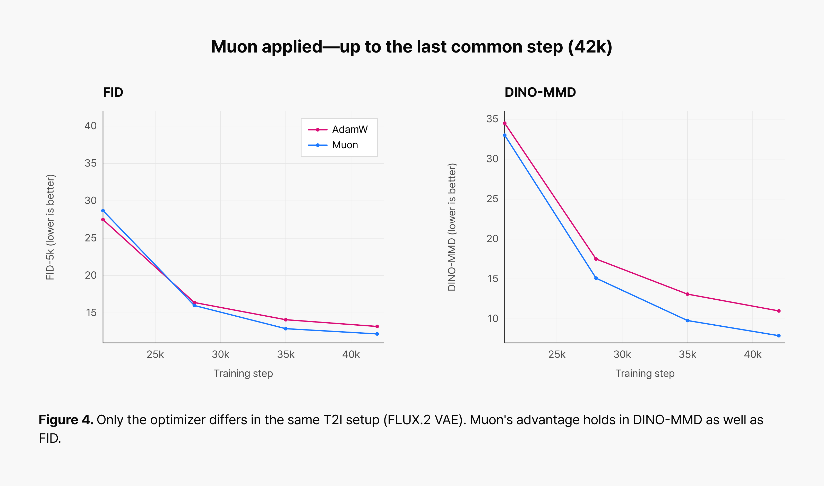
The T2I experiments, which generate images from natural-language prompts, showed the same trend. At the last common step (42k), the setup with the FLUX.2 VAE scored 13.19 on FID and 11.05 on DINO-MMD. Changing only the optimizer to Muon brought those to 12.07 and 7.96. Muon’s advantage held not just under simple category conditioning but with real sentences as input.
Is the best noise setting for training also the best for generation?
An image generation model starts from formless noise and builds an image by reducing that noise over many steps. Flow matching [9] learns the path from pure noise to a clean image, at many points along the way. The model sees a range of inputs, from heavily noised states to states close to a finished image, and learns which direction to move at each point.
The noise shift determines which noise range the model trains on most often. In this setup, a larger shift puts relatively more weight on the noisier range and a smaller shift on the cleaner range. That choice shapes the difficulty of the problems the model meets most often during training.
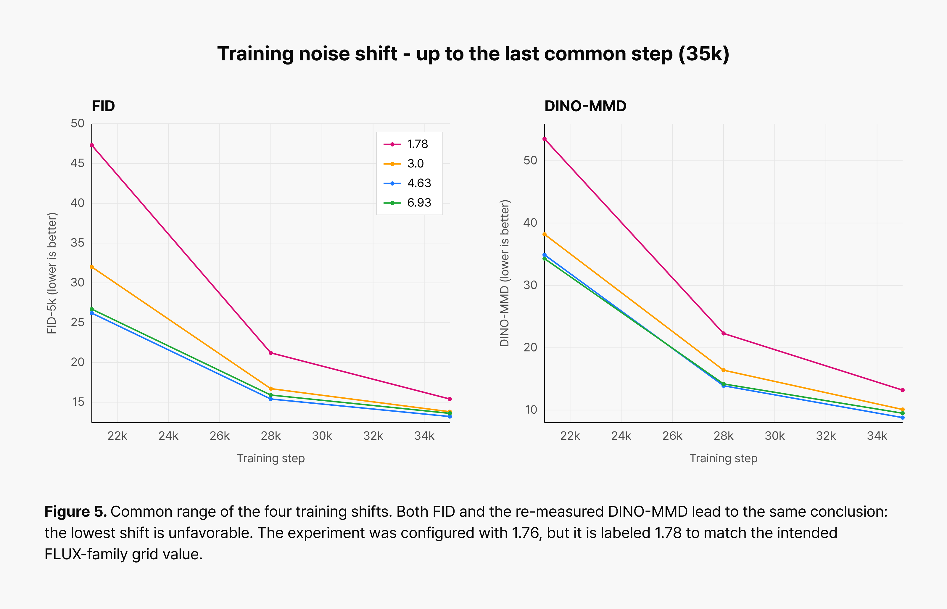
We compared four training shifts first. Only the lowest value came out clearly worse; the mid-range values performed about the same. We also tried logit-normal, plateau, and uniform distributions for sampling the timestep to train on, but the differences were small.
Changing only the shift used to generate images from a trained model told a different story. Across the 1.78–6.93 range we tested, FID fell as the generation shift went up.
This shows that a setting that’s good for training isn’t automatically good for the generation process. The training shift determines which noise range the model centers its learning on; the generation shift tunes how a trained model builds an image. Their roles differ, so it made more sense to tune the two separately than to lock them to a single value.
Can understanding an image improve generation quality?
The generation loss alone is enough for a model to learn how to move a noisy latent representation toward a clean image. It’s harder to guarantee, though, that this alone builds an internal representation of what’s in the image and how the elements are arranged. Earlier work has shown that internal representations carrying good semantic information help image generation [10, 11].
A common approach to train such representations is representation alignment. REPA [12] aligns the intermediate features of a Diffusion Transformer with representations from an external visual encoder pretrained to capture semantics well.
Self-Flow [13], the method we applied, uses no external encoder. It takes an exponential moving average (EMA) copy of the model being trained as the teacher instead.
The teacher sees a less noisy input from the same image, while the student sees an input with some tokens corrupted more heavily. Taking the teacher’s representation as its target, the student learns to recover the meaning and structure of the cleaner input even from a noisier state. The model learns to understand images as well as generate them.
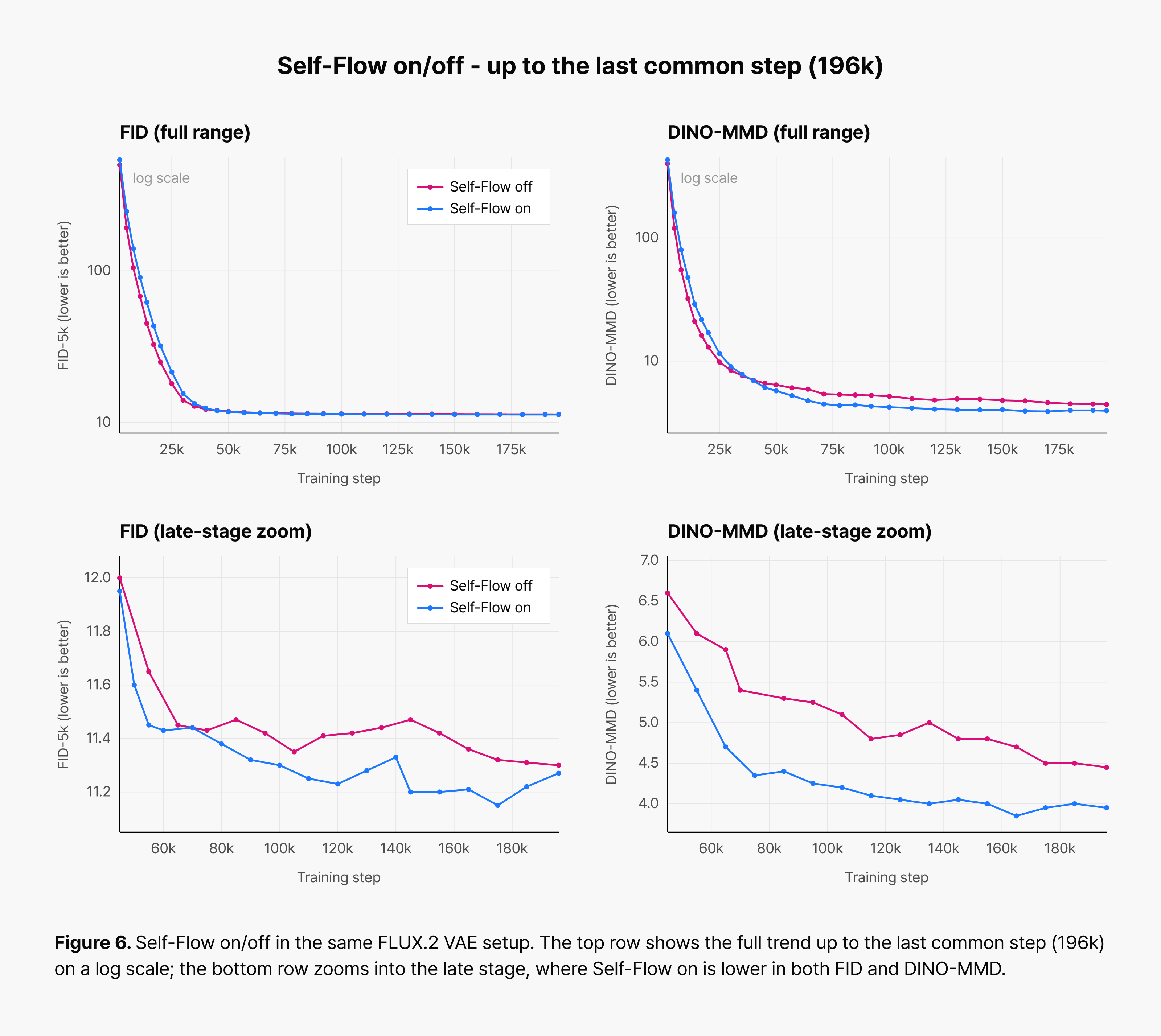
We started by adding Self-Flow to the 42k-step T2I setup with the FLUX.2 VAE and Muon. FID stayed about the same, moving from 12.07 to 12.41, but DINO-MMD fell from 7.96 to 7.01. Over a short training run, FID alone wasn’t enough to judge the benefit, but DINO-MMD, which compares image distributions in DINO’s feature space, picked up the improvement first.
To see whether Self-Flow’s effect became clearer later in training, we trained both setups out to 196k steps. At 147k steps, FID was 11.47 with Self-Flow off and 11.25 with it on; DINO-MMD was 4.85 and 4.05. At 196k steps the FID gap was small, 11.30 against 11.27, but DINO-MMD fell from 4.46 to 3.91. Later in training, the Self-Flow setup generally came out lower on FID too.
This pattern—the benefit sharpening once training has run long enough—matches trends reported in some of the experiments in the Self-Flow paper [13]. Self-Flow kept improving after the comparison methods had plateaued, and confirming the benefit took a longer run.
We didn’t draw a conclusion from a single FID point over a short run either. Looking at the late-training curves together with DINO-MMD, we judged that Self-Flow’s advantage emerges as training gets longer, and included it in the final recipe.
What keeps early information from fading?
An image generation model processes its input in stages, block by block. Along the way, information an early block picked up—position, edges—can weaken before it reaches the later blocks. A long skip lets later blocks directly access features from earlier blocks, in addition to the normal path through the intermediate blocks.
U-Net [14] is what made this approach widely known. U-Net passes feature maps from the front of the encoder directly to the matching decoder layer, so that position and edge information that can fade going through the bottleneck in the middle is available again when the image is reconstructed.
U-ViT [15] later applied long skips to Diffusion Transformers, connecting shallow and deep layers symmetrically. It has no downsampling/upsampling path like U-Net’s, but this showed that the connection itself—passing early information straight through to the back—can help generation performance.
More recently, i1 [16] revisited the design in a modern T2I backbone and found consistent benefits across several model sizes and architectures. We applied long skips as well, so that later blocks can directly reuse the spatial information and text conditioning formed in the earlier transformer blocks. Image tokens and text tokens travel together between symmetric front and back blocks.
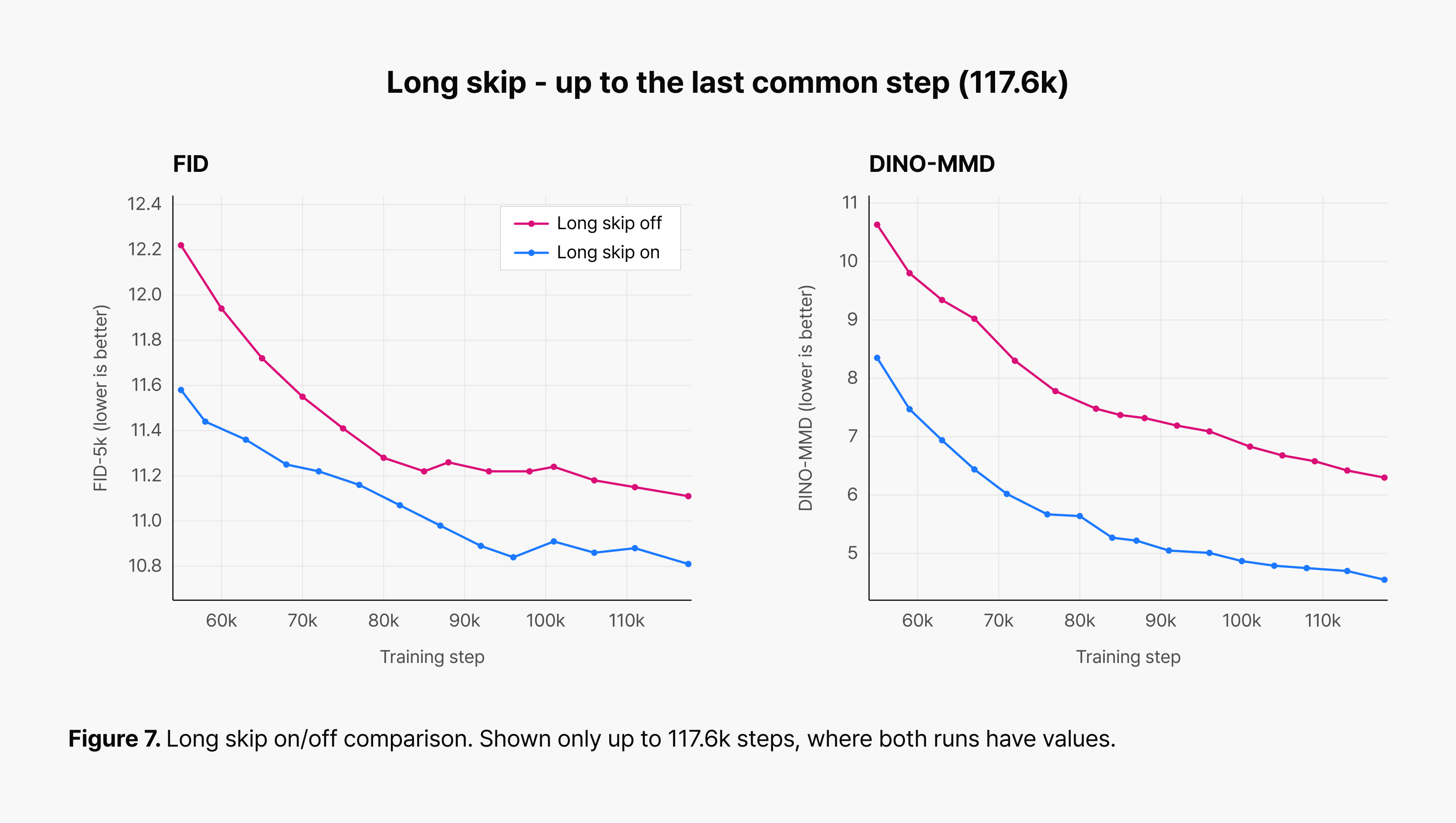
To isolate the effect of the long skip itself, we held everything else constant and compared it on and off. At the last common step (117.6k), FID was 11.11 with long skips off and 10.81 with them on. Re-measured DINO-MMD for the same setups was 6.30 and 4.53.
The FID gap looks small, but DINO-MMD, which compares image distributions in a different visual representation space, showed a clearer improvement. Both metrics confirmed that passing early-block information straight to the back still works in this model.
What does text rendering reveal about how a model reads prompts?
For a T2I model to build the image a user asked for, it has to get the prompt’s meaning right. The text encoder parses the sentence and passes the resulting hidden states to the image generation model as conditioning.
Not every layer of the text encoder holds the same information, though. How abstract or how detailed a representation is can vary with layer depth. We suspected that the information needed to understand a prompt’s overall meaning and the information needed to render the fine shapes of letters inside an image might sit at different depths.
This model uses a vision-language model (VLM) as its text encoder. We compared using only the VLM’s final layer against concatenating representations from several intermediate layers.
Using representations from different depths together held up on standard T2I evaluation as well. The difference was sharpest in text rendering—generating letters inside the image.
Models using a single layer’s representation sometimes misspelled words or doubled a letter. Models using representations from several depths generated letters more accurately after the same number of training steps. A difference barely visible in the training loss or the overall averages showed up immediately in the actual images.
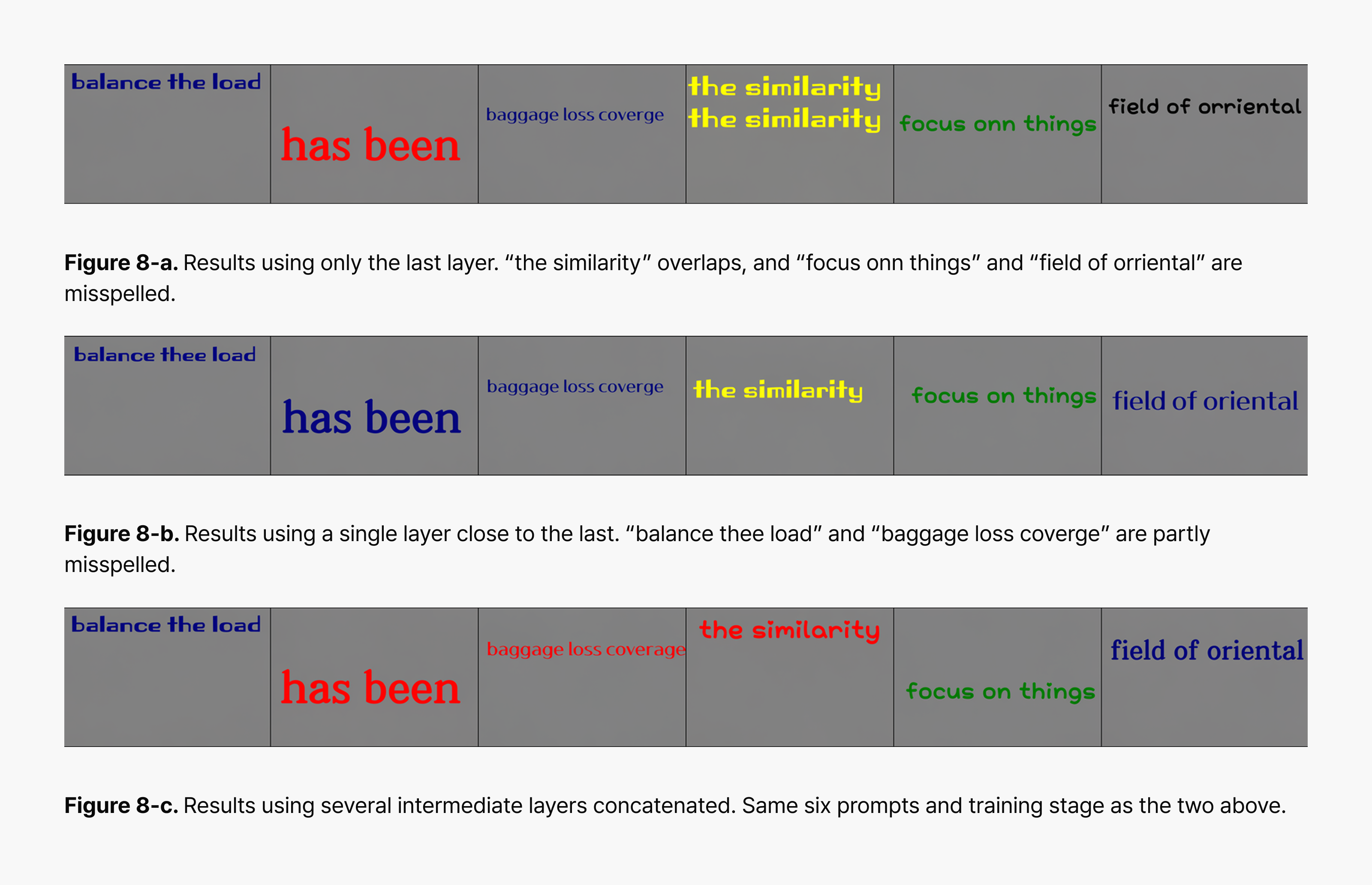
This experiment showed us that text rendering can be a sensitive yardstick for differences in text conditioning. With ordinary generated images, composition and texture vary, which can make it hard to say which result is better. But a single wrong letter makes the difference unmistakable.
So for a model that has to read text accurately and render it inside an image, text rendering results deserve a look alongside overall average scores. On that basis, we put the text conditioning structure that uses several of the VLM’s intermediate layers into the final recipe.
3. The techniques we didn’t adopt pointed to the next question
The techniques we didn’t adopt mattered as much as the ones we did. Rather than sorting results into “worked” and “didn’t work,” we recorded both our judgment under current conditions and what would make us check again.
Does predicting the clean image directly help the model learn?
Flow matching training normally predicts velocity—the direction to move from the current noisy state toward the clean image (v-prediction). JiT [17], on the other hand, changes the objective so the model predicts the clean image’s raw pixel values directly instead of a direction (x₀-prediction).
JiT is motivated by the high dimensionality of pixel space. A 256×256 color image consists of roughly 200,000 values, but natural images do not occupy this entire space; instead, they are concentrated in a structured, low-dimensional region. JiT therefore argues that learning can be more efficient when the model directly predicts a clean image in this low-dimensional region, rather than predicting noise or velocity targets that are not confined to the same region.
We first kept our existing VAE latent space and changed only the prediction objective to x₀-prediction, following JiT. Because the VAE-compressed latent representation has different low-dimensional characteristics from pixel space, we did not observe the sharp degradation of v-prediction reported by JiT in pixel space. Both objectives trained stably, and v-prediction actually performed slightly better than x₀-prediction.
Since this result was unexpected, we ran the experiment again after removing the VAE. This time, we observed a result similar to the JiT paper: x₀-prediction clearly outperformed v-prediction.
These two experiments reinforced an important lesson: even techniques that work well individually do not necessarily retain the same benefits when combined. JiT itself was a valid approach, but it did not provide an advantage when combined with our VAE setup, so we left it out of the final recipe.
Register tokens worked as intended, but quality didn’t follow
A Vision Transformer splits an image into patches and processes each patch as a token. “Vision Transformers Need Registers” [18] reported that abnormally large tokens—high-norm tokens—appear in low-information background patches.
Rather than representing the content of the surrounding image, these tokens were being used as scratch space for information the model needed for its internal computation. Tokens meant to hold image information were taking on another role.
Register tokens are a way to add separate learnable tokens dedicated to that internal computation. The aim is to keep image tokens from having to double as storage for internal information, so each patch’s content is represented more faithfully.
“F Lite Technical Report” [19] later applied this to a large-scale T2I Diffusion Transformer. Register tokens are prepended to the image-token sequence so that they participate in self-attention, and are discarded before the final image-token outputs are produced.
Following that example, we added 8 and 16 register tokens and compared against the baseline. Attention did in fact concentrate on the new tokens, so the mechanism checked out: the model does use register tokens as internal scratch space.
But tokens working as intended and generated images getting better were separate questions. At 140k steps the FID difference between setups was 0.059, smaller than the observed measurement variation, and DINO-MMD showed no consistent improvement.
Recent work [20] also found that register tokens give their largest improvement in pixel space, with a relatively smaller gain in VAE latent space—the same direction as our result, where register tokens offered little benefit in latent-space experiments. That said, the models and training conditions in that work differ from ours, so we treated it as support for our reading rather than a direct cause of the result.
Does a longer-lasting training signal buy better representations?
One thing we noticed while training Self-Flow: the alignment loss, which measures the gap between the student’s and the teacher’s representations, dropped fast early in training and then barely moved.
Standard Self-Flow aligns the two representations based on whether they point in the same direction. Would changing the alignment so the loss didn’t shrink this early keep a more useful signal alive later in training?
First we applied DINO-style [21] distribution alignment. This converts the teacher and student representations into probability distributions and aligns their output distributions. The teacher’s distribution is then sharpened to provide a more specific target for the student.
The intended change did happen. The steep early drop in alignment loss disappeared, and the training signal held up later in training. But the change in the loss curve didn’t translate into better images.
At 196k steps, the FID difference between standard Self-Flow and the new alignment was just 0.023. Qualitative comparison gave no clear winner either, and DINO-MMD showed no consistent difference large enough to justify adopting the new approach.
This experiment showed that a longer-lasting alignment signal does not necessarily mean that the model learns more useful representations. A change in an optimization metric does not guarantee an improvement in final generation quality.
The second thing we looked at, iREPA [22], aligns representations while preserving spatial information that can disappear when a whole image is pooled into a single vector. But at 117.6k steps the quality difference wasn’t clear, and in some setups the computational cost rose sharply.
Under current conditions we didn’t find a benefit worth the extra structure and compute, so the final recipe keeps standard Self-Flow. We’ve left iREPA as a candidate to revisit if we improve its implementation efficiency, or once the model scales up or input sequences get longer.
Scaling up the architecture isn’t always the answer
We also tried scaling up the structure that handles text conditioning. A T2I model has to convert the representations produced by the text encoder into a form the image generation model can use. The module that does this is the adapter.
i1 [16] proposed building the adapter from Transformer blocks rather than a simple multilayer perceptron (MLP), increasing its capacity to process text conditioning. We applied this too, but at our current scale the separate module and extra compute didn’t pay for themselves. We’ll revisit it in a setting where text conditioning capacity is the actual performance bottleneck.
We also compared shared and sandwich normalization. The results changed little, but we did not take this as evidence that normalization techniques are ineffective in general. The original study evaluated these techniques in combination with RMSNorm, whereas we implemented them using LayerNorm in a backbone that retained AdaLN. We interpreted this result as indicating that these techniques were a lower priority for our current configuration, rather than as a judgment on their general usefulness.
Beyond that, we varied the ratio of blocks that process text and image tokens separately to blocks that process them jointly. We also compared Contrastive Flow Matching [23], which more strongly separates the generation paths that different captions produce.
Some setups improved the image distribution but scored worse on prompt adherence. Others grew the architecture and compute cost more than they moved the evaluation metrics. We didn’t pick a technique on one metric alone; we weighed image quality, prompt adherence, and compute cost together.
These experiments weren’t just a list of failures. With register tokens, the mechanism checked out but quality didn’t improve. With DINO-style alignment, the training signal changed but the final result didn’t. With JiT, we changed the model’s representation space and prediction target to test the core configuration of the original paper, but under our experimental conditions, the gains were not clear enough to justify including it in the final recipe.
That gave us a record not just of what we wouldn’t adopt, but of why, and under what conditions to check again. Records like these let the next model start without repeating the same experiments from scratch, and help us pick suitable candidates quickly.
4. Do good choices add up to a good recipe?
Adding up every technique that worked in an individual ablation doesn’t produce a finished recipe. Each did well on its own, but used together, effects can overlap or interfere.
Changing one element can also change what the right value is for another. Swap the VAE or the image resolution, for instance, and the shape and statistics of the data change, which means the noise shift needs retuning too.
So we didn’t just sum up the individual results. We added each validated technique one at a time and rechecked that its benefit survived in combination.
First, in the same T2I setup, we applied the FLUX.2 VAE and then Muon, comparing at the last common step (42k). Self-Flow improved DINO-MMD first in the short runs, but its FID difference wasn’t clear, so we trained both FLUX.2 VAE setups out to 196k steps before judging.
The table below shows the before-and-after change for the three techniques we could compare quantitatively. Rather than adding up numbers from different training steps, we compared each experiment at the last common step.
| Single change | Common step | FID-5k (before → after) ↓ | DINO-MMD (before → after) ↓ |
|---|---|---|---|
| (a): FLUX.1 VAE → FLUX.2 VAE | 42k | 35.12 → 13.19 | 37.77 → 11.05 |
| (b): (a) + AdamW → Muon | 42k | 13.19 → 12.07 | 11.05 → 7.96 |
| (c): (b) + Self-Flow | 196k | 11.30 → 11.27 | 4.46 → 3.91 |
In a second round of combined validation, we added only the long skip to a shared setup that used several of the VLM’s intermediate layers. At 117.6k steps, FID fell from 11.11 to 10.81, while DINO-MMD fell from 6.30 to 4.53. The benefit of the long skip therefore remained even after it was combined with the techniques selected in the preceding validation and the chosen text-conditioning setup. Rather than collapsing results from separate validation runs into a single aggregate score, we checked sequentially whether each newly added choice retained its benefit after the techniques were combined. We tuned the noise shift separately for training and generation, and selected the text-conditioning setup based on both standard T2I metrics and text-rendering results.
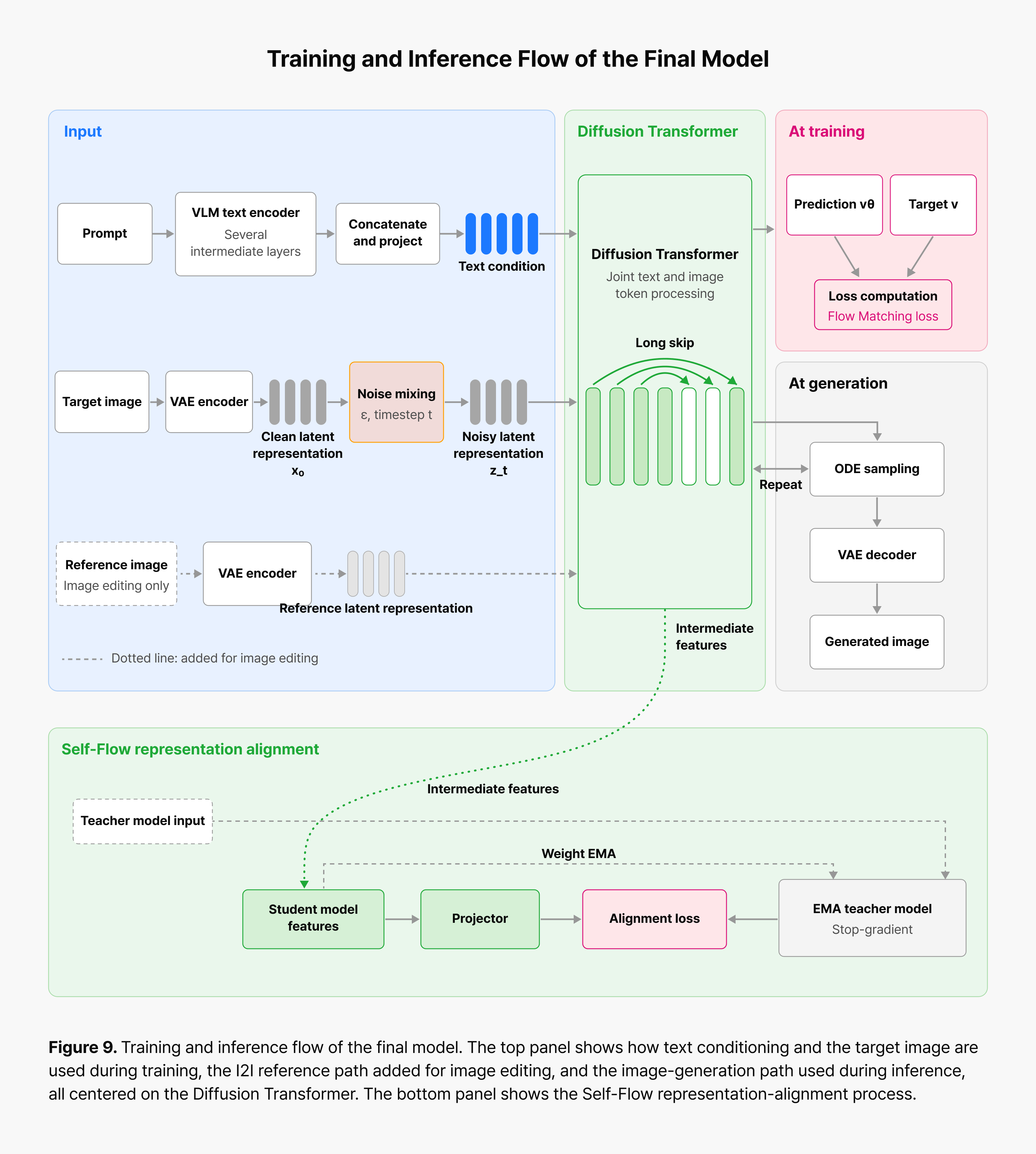
Combining all of this gave us one training recipe: a latent representation suited to generation, a noise shift matched to the data statistics, Muon, Self-Flow, long skips, and text conditioning drawing on several of the VLM’s intermediate layers.
The result showed promise not just in general image generation but in following complex descriptive prompts and in Korean and English text rendering. We also extended it to image editing, our original goal, establishing a base for changing the parts you specify while keeping the original context.
Some areas aren’t solved by architecture search alone, though. Human aesthetic preference and fine texture depend heavily on data composition and post-training. We’re improving that area separately from the architecture search covered here, raising perceived quality through post-training that includes reinforcement learning, where human preference over generated results is defined as the reward.

5. From research result to real service
Building on these research results, we’re also preparing to connect the model to actual NAVER services. We’re looking at uses ranging from creating an image for a work document or presentation and then editing just the parts you want, to quickly producing multiple ad variations by changing backgrounds and copy.
In a real service, being able to produce one plausible image isn’t enough. The model has to read the user’s instruction accurately and tell apart what should stay from what should change. It must also maintain consistent quality across repeated requests.
In settings where accuracy and consistency matter—companies and public institutions especially—these conditions tie directly to trust in the model. Results have to reflect the user’s intent reliably and stand up to repeated use in real work.
By improving instruction understanding and editing consistency alongside generation quality, we want to carry the technical foundation from this research into real NAVER services.
6. Closing thoughts
The biggest result from this work wasn’t a list of settings that apply to one particular model. It was a repeatable search method for validating new candidates quickly and finding the choices that fit current conditions.
Research moves fast, so we picked out promising techniques and tested them on small models, one element at a time. We compared wall-clock time as well as training steps, and looked at several quantitative metrics and the generated images themselves rather than leaning on FID alone.
We didn’t throw out the experiments whose differences weren’t clear. We recorded why we hadn’t adopted them under current conditions and what conditions would warrant another look. That let us focus on choices that actually hold up in the current model, instead of adding every new technique that comes along.
Many of the final recipe’s choices differed from what our literature review and early discussions had predicted. In some cases, the latent representation, the optimizer, and training settings matched to the data made more difference than complicating the architecture. Techniques with good results in papers shifted in priority once model size, resolution, and training space changed.
One evaluation method wasn’t enough either. Differences FID didn’t capture well came through in DINO-MMD and text rendering. We examined details the quantitative metrics miss—text, fingers, repeating patterns—by directly comparing images generated from the same prompts.
“Change the background to a hanok, a traditional Korean house, have both people hold coffee, and add sunglasses to the man.”
What does a model need to learn first to follow an instruction like this?
In the end, this isn’t achieved by training on editing data alone. A latent space that represents images effectively, text conditioning that understands complex instructions, and an architecture that can learn enough within a limited time all have to be in place first.
On that foundation, NAVER Cloud aims to develop an image generation and editing model that understands Korean instructions accurately and naturally renders the visual context familiar to Korean users.
Drawing a complex scene described in Korean the way it was intended, rendering the copy inside a poster accurately, and changing the background, props, and subject attributes in a single edit while keeping the whole scene natural—we’ll keep looking for better architectures and training methods until generation and editing like this become tools anyone can trust and use, not a special feature.
References and open implementations
[1] Martin Heusel et al., “GANs Trained by a Two Time-Scale Update Rule Converge to a Local Nash Equilibrium,” NeurIPS 2017. https://arxiv.org/abs/1706.08500 · FID code: https://github.com/bioinf-jku/TTUR
[2] Maxime Oquab et al., “DINOv2: Learning Robust Visual Features without Supervision,” TMLR 2024. https://arxiv.org/abs/2304.07193 · Code: https://github.com/facebookresearch/dinov2
[3] PhotoRoom, “PRX: An Open-Source Text-to-Image Model,” evaluation implementation including DINO-MMD, 2026. https://github.com/Photoroom/PRX
[4] Alec Radford et al., “Learning Transferable Visual Models From Natural Language Supervision,” ICML 2021. https://arxiv.org/abs/2103.00020 · Code: https://github.com/openai/CLIP
[5] Christoph Schuhmann, “CLIP+MLP Aesthetic Score Predictor (LAION Aesthetic Predictor V2),” 2022. https://github.com/christophschuhmann/improved-aesthetic-predictor
[6] Black Forest Labs, “FLUX.2: Analyzing and Enhancing the Latent Space of FLUX — Representation Comparison,” 2025. https://bfl.ai/research/representation-comparison
[7] Ilya Loshchilov and Frank Hutter, “Decoupled Weight Decay Regularization,” ICLR 2019. https://arxiv.org/abs/1711.05101 · Code: https://github.com/loshchil/AdamW-and-SGDW
[8] Keller Jordan et al., “Muon: An Optimizer for Hidden Layers in Neural Networks,” 2024. https://kellerjordan.github.io/posts/muon/ · Code: https://github.com/KellerJordan/Muon
[9] Yaron Lipman et al., “Flow Matching for Generative Modeling,” ICLR 2023. https://arxiv.org/abs/2210.02747
[10] Alexey Dosovitskiy and Thomas Brox, “Generating Images with Perceptual Similarity Metrics based on Deep Networks,” NeurIPS 2016. https://arxiv.org/abs/1602.02644
[11] Tim Salimans et al., “Improved Techniques for Training GANs,” NeurIPS 2016. https://arxiv.org/abs/1606.03498
[12] Sihyun Yu et al., “Representation Alignment for Generation: Training Diffusion Transformers Is Easier Than You Think,” ICLR 2025. https://arxiv.org/abs/2410.06940
[13] Hila Chefer et al., “Self-Supervised Flow Matching for Scalable Multi-Modal Synthesis,” 2026. https://arxiv.org/abs/2603.06507 · Code: https://github.com/black-forest-labs/Self-Flow
[14] Olaf Ronneberger, Philipp Fischer, and Thomas Brox, “U-Net: Convolutional Networks for Biomedical Image Segmentation,” MICCAI 2015. https://arxiv.org/abs/1505.04597
[15] Fan Bao et al., “All are Worth Words: A ViT Backbone for Diffusion Models,” CVPR 2023. https://arxiv.org/abs/2209.12152 · Code: https://github.com/baofff/U-ViT
[16] Boya Zeng et al., “i1: A Simple and Fully Open Recipe for Strong Text-to-Image Models,” 2026. https://arxiv.org/abs/2606.11289 · Code: https://github.com/zlab-princeton/i1
[17] Tianhong Li and Kaiming He, “Back to Basics: Let Denoising Generative Models Denoise,” 2025. https://arxiv.org/abs/2511.13720
[18] Timothée Darcet et al., “Vision Transformers Need Registers,” ICLR 2024. https://arxiv.org/abs/2309.16588
[19] Simo Ryu, Lu Pengqi, Javier Martín Juan, and Iván de Prado Alonso, “F Lite Technical Report,” 2025. https://github.com/fal-ai/f-lite/blob/main/assets/F%20Lite%20Technical%20Report.pdf · Code: https://github.com/fal-ai/f-lite
[20] Nikita Starodubcev et al., “Registers Matter for Pixel-Space Diffusion Transformers,” 2026. https://arxiv.org/abs/2605.16147
[21] Mathilde Caron et al., “Emerging Properties in Self-Supervised Vision Transformers,” ICCV 2021. https://arxiv.org/abs/2104.14294
[22] Jaskirat Singh et al., “What Matters for Representation Alignment: Global Information or Spatial Structure?,” 2025. https://arxiv.org/abs/2512.10794 · Code: https://github.com/end2end-diffusion/irepa
[23] George Stoica et al., “Contrastive Flow Matching,” ICCV 2025. https://arxiv.org/abs/2506.05350 · Code: https://github.com/gstoica27/DeltaFM